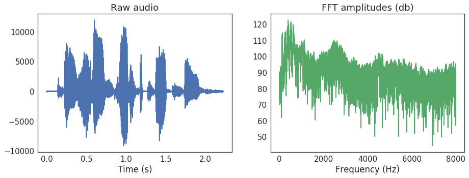
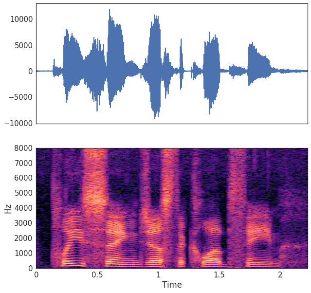
The spectrogram - spectral changes to sound over time

Machine Learning for Time Series Data in Python

Chris Holdgraf

Fellow, Berkeley Institute for Data Science

Fourier transforms

  • Timeseries data can be described as a combination of quickly-changing things and slowly-changing things
  • At each moment in time, we can describe the relative presence of fast- and slow-moving components
  • The simplest way to do this is called a Fourier Transform
  • This converts a single timeseries into an array that describes the timeseries as a combination of oscillations
Machine Learning for Time Series Data in Python

A Fourier Transform (FFT)

Machine Learning for Time Series Data in Python

Spectrograms: combinations of windows Fourier transforms

  • A spectrogram is a collection of windowed Fourier transforms over time
  • Similar to how a rolling mean was calculated:
    1. Choose a window size and shape
    2. At a timepoint, calculate the FFT for that window
    3. Slide the window over by one
    4. Aggregate the results
  • Called a Short-Time Fourier Transform (STFT)
Machine Learning for Time Series Data in Python

Machine Learning for Time Series Data in Python

Calculating the STFT

  • We can calculate the STFT with librosa
  • There are several parameters we can tweak (such as window size)
  • For our purposes, we'll convert into decibels which normalizes the average values of all frequencies
  • We can then visualize it with the specshow() function
Machine Learning for Time Series Data in Python

Calculating the STFT with code

# Import the functions we'll use for the STFT
from librosa.core import stft, amplitude_to_db
from librosa.display import specshow
import matplotlib.pyplot as plt

# Calculate our STFT
HOP_LENGTH = 2**4
SIZE_WINDOW = 2**7
audio_spec = stft(audio, hop_length=HOP_LENGTH, n_fft=SIZE_WINDOW)

# Convert into decibels for visualization
spec_db = amplitude_to_db(audio_spec)

# Visualize
fig, ax = plt.subplots()
specshow(spec_db, sr=sfreq, x_axis='time', 
         y_axis='hz', hop_length=HOP_LENGTH, ax=ax)
Machine Learning for Time Series Data in Python

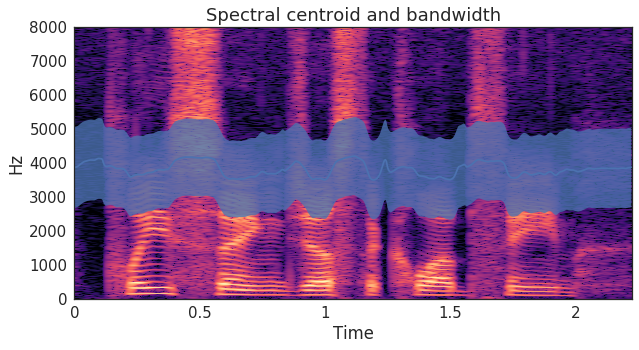
Spectral feature engineering

  • Each timeseries has a different spectral pattern.
  • We can calculate these spectral patterns by analyzing the spectrogram.
  • For example, spectral bandwidth and spectral centroids describe where most of the energy is at each moment in time

Machine Learning for Time Series Data in Python

Calculating spectral features

# Calculate the spectral centroid and bandwidth for the spectrogram
bandwidths = lr.feature.spectral_bandwidth(S=spec)[0]
centroids = lr.feature.spectral_centroid(S=spec)[0]

# Display these features on top of the spectrogram
fig, ax = plt.subplots()
specshow(spec, x_axis='time', y_axis='hz', hop_length=HOP_LENGTH, ax=ax)
ax.plot(times_spec, centroids)
ax.fill_between(times_spec, centroids - bandwidths / 2, 
                centroids + bandwidths / 2, alpha=0.5)
Machine Learning for Time Series Data in Python

Combining spectral and temporal features in a classifier

centroids_all = []
bandwidths_all = []
for spec in spectrograms:
    bandwidths = lr.feature.spectral_bandwidth(S=lr.db_to_amplitude(spec))
    centroids = lr.feature.spectral_centroid(S=lr.db_to_amplitude(spec))
    # Calculate the mean spectral bandwidth
    bandwidths_all.append(np.mean(bandwidths))  
    # Calculate the mean spectral centroid
    centroids_all.append(np.mean(centroids))  

# Create our X matrix
X = np.column_stack([means, stds, maxs, tempo_mean, 
                     tempo_max, tempo_std, bandwidths_all, centroids_all])
Machine Learning for Time Series Data in Python

Let's practice!

Machine Learning for Time Series Data in Python

Preparing Video For Download...