การตีความผลลัพธ์และการเปรียบเทียบโมเดล

การวิเคราะห์ข้อมูลแบบเบย์เซียนด้วย Python

Michal Oleszak

Machine Learning Engineer

ทบทวนการรันโมเดล

formula = "num_clicks ~ clothes_banners_shown + sneakers_banners_shown"

with pm.Model() as model_1:
    pm.GLM.from_formula(formula, data=ads_aggregated)
    trace_1 = pm.sample(draws=1000, tune=500)

ทบทวนการรันโมเดล

formula = "num_clicks ~ clothes_banners_shown + sneakers_banners_shown"

with pm.Model() as model_1:
    pm.GLM.from_formula(formula, data=ads_aggregated)
    trace_1 = pm.sample(draws=1000, tune=500, chains=4)

จำนวนพารามิเตอร์: 4
จำนวน draws ต่อพารามิเตอร์: 1000 $\times$ 4 = 4000

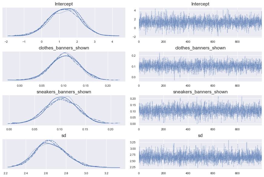
Trace plot

pm.traceplot(trace_1)

กริดของกราฟแปดช่องสองคอลัมน์สี่แถว คอลัมน์ซ้ายมีกราฟความหนาแน่นสี่กราฟ คอลัมน์ขวามีกราฟเส้นสี่กราฟ แต่ละกราฟแสดงพารามิเตอร์หนึ่งตัว

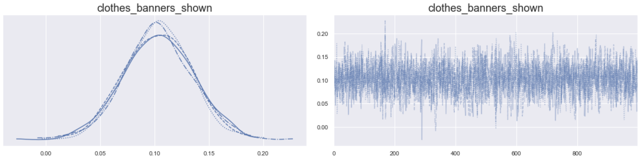
Trace plot: ขยายดูพารามิเตอร์เดียว

กราฟสองช่องเคียงกัน ซ้ายเป็นกราฟความหนาแน่น ขวาเป็นกราฟเส้นแสดง draws ของพารามิเตอร์

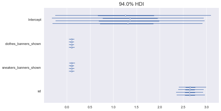
Forest plot

pm.forestplot(trace_1)

กราฟแสดงการกระจายตัวของ draws สำหรับพารามิเตอร์แต่ละตัวในรูปแบบแนวนอน

Trace summary

pm.summary(trace_1)

                         mean     sd  hdi_3%  hdi_97%  mcse_mean  mcse_sd  \
Intercept               1.307  0.886  -0.305    2.962      0.018    0.013   
clothes_banners_shown   0.103  0.031   0.043    0.160      0.001    0.000   
sneakers_banners_shown  0.104  0.032   0.045    0.163      0.001    0.001   
sd                      2.654  0.157   2.382    2.970      0.003    0.002   

                        ess_mean  ess_sd  ess_bulk  ess_tail  r_hat  
Intercept                 2346.0  2318.0    2351.0    2083.0    1.0  
clothes_banners_shown     2085.0  2085.0    2089.0    1868.0    1.0  
sneakers_banners_shown    2105.0  1953.0    2122.0    1869.0    1.0  
sd                        2615.0  2590.0    2646.0    1834.0    1.0

ฟิตโมเดลอีกตัว

formula = "num_clicks ~ clothes_banners_shown + sneakers_banners_shown + weekend"

with pm.Model() as model_2:
    pm.GLM.from_formula(formula, data=ads_aggregated)
    trace_2 = pm.sample(draws=1000, tune=500)

Widely Applicable Information Criterion (WAIC)

comparison = pm.compare({"trace_1": trace_1, "trace_2": trace_2}, 
                        ic="waic", scale="deviance")
print(comparison)

        rank     waic   p_waic    d_waic    weight       se      dse warning  \
trace_2    0   -362.8   5.1576         0  0.513792  9.37269        0    True   
trace_1    1 -362.926  4.13318  0.126236  0.486208  9.48352  1.50682    True   

        waic_scale  
trace_2        log  
trace_1        log

Compare plot

pm.compareplot(comparison)

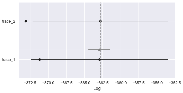
กราฟแสดงค่า WAIC ของโมเดลสองตัว

มาฝึกกันเถอะ!

การวิเคราะห์ข้อมูลแบบเบย์เซียนด้วย Python