Konvex optimering med olikhetsbetingelser

Introduktion till optimering i Python

Jasmin Ludolf

Content Developer

Hörnlösning kontra inre lösning
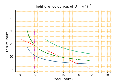
  • Alexia har bara 5 timmars arbete

$$ w\leq 5$$

  • Två betingelser:
    • 24 timmar per dygn
    • 5 timmars arbete
  • Betingelserna bildar ett hörn
  • Inre lösningen är ingen skärningspunkt

Indifferenskurvor och betingelser. Indifferenskurvan vid optimal nyttanivå passerar genom skärningspunkten för betingelserna.

Introduktion till optimering i Python

Tillverkare med kapacitetsbetingelser

  • Biltillverkaren producerar identiska bilar i två fabriker $A$, $B$
    • Kvantiteter: $q_A$, $q_B$
    • Kapacitet: $q_A\leq 90$, $q_B\leq 90$
    • Kostnad: $C_A(q)=3q$, $C_B(q)=3.5q$
  • Efterfrågan:
    • $P=120-Q$
  • Kontrakt:
    • $Q\geq 92$
  • Mål – maximera vinst:
    • $\displaystyle\max \Pi(q_A,q_B)$

Biltillverkningslinje

Introduktion till optimering i Python

Vinstmaximering

  • Mål:
    • $\Pi = R-C$
      • $R = PQ$
Introduktion till optimering i Python

Vinstmaximering

  • Mål:
    • $\Pi = R-C$
      • $R = PQ = (120-Q)Q $
Introduktion till optimering i Python

Vinstmaximering

  • Mål:

    • $\Pi = R-C$
      • $R = PQ = (120-Q)Q=\left[120-(q_A+q_B)\right](q_A+q_B)$
      • $C=C_A+C_B=3q_A+3.5q_B$
  • Gränser

    • $0\leq q_A, q_B\leq 90$
  • Betingelser
    • $Q\geq92\Leftrightarrow 92\leq q_A+q_B$
Introduktion till optimering i Python

Formulering

$$\max_{q_A,q_B}R(q_A,q_B)-C(q_A,q_B)$$

$$s.t.$$

$$R(q_A,q_B)=\left[120-(q_A+q_B)\right](q_A+q_B)$$

$$\ \ \ \ \ C(q_A,q_B)=3q_A+3.5q_B$$

$$\ \ \ 0\leq q_A, q_B\leq 90$$

$$ \ \ \ \ 92\leq q_A+q_B$$

from scipy.optimize import minimize,\
        Bounds, LinearConstraint


def R(q): return (120 - (q[0] + q[1] )) * (q[0] + q[1])
def C(q): return 3*q[0] + 3.5*q[1]
def profit(q): return R(q) - C(q)
bounds = Bounds([0, 0], [90, 90])
constraints = LinearConstraint([1, 1], lb=92)
Introduktion till optimering i Python

Maximera vinst med SciPy

result = minimize(lambda q: -profit(q),

[50, 50],
bounds=bounds, constraints=constraints)
print(result.message) print(f'The optimal number of cars produced in plant A is: {result.x[0]:.2f}') print(f'The optimal number of cars produced in plant B is: {result.x[1]:.2f}') print(f'The firm made: ${-result.fun:.2f}')
Optimization terminated successfully
The optimal number of cars produced in plant A is: 90.00
The optimal number of cars produced in plant B is: 2.00
The firm made: $2299.00
Introduktion till optimering i Python

Icke-linjära betingelser i SciPy

from scipy.optimize import NonlinearConstraint 
import numpy as np


constraints = NonlinearConstraint(lambda q: q[0] + q[1], lb=92, ub=np.inf)
result = minimize(lambda q: -profit(q), [50, 50], bounds=Bounds([0, 0], [90, 90]), constraints=constraints)
Introduktion till optimering i Python

Lösning med NonlinearConstraint

print(result.message)
print(f'The optimal number of cars produced in plant A is: {result.x[0]:.2f}')
print(f'The optimal number of cars produced in plant B is: {result.x[1]:.2f}')
print(f'The firm made: ${-result.fun:.2f}') 
Optimization terminated successfully
The optimal number of cars produced in plant A is: 90.00
The optimal number of cars produced in plant B is: 2.00
The firm made: $2299.00 
  • Använd LinearConstraint() för enkla, linjära problem
  • Annars, använd NonlinearConstraint()
Introduktion till optimering i Python

Nu kör vi en övning!

Introduktion till optimering i Python

Preparing Video For Download...