Inferens för kategoriska data i R
Andrew Bray
Assistant Professor of Statistics at Reed College
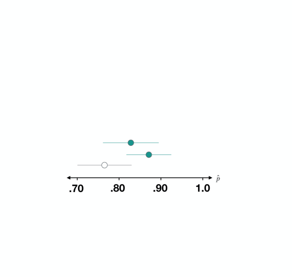
Slutsats: den sanna andelen amerikaner som är lyckliga ligger mellan 0,705 och 0,841.
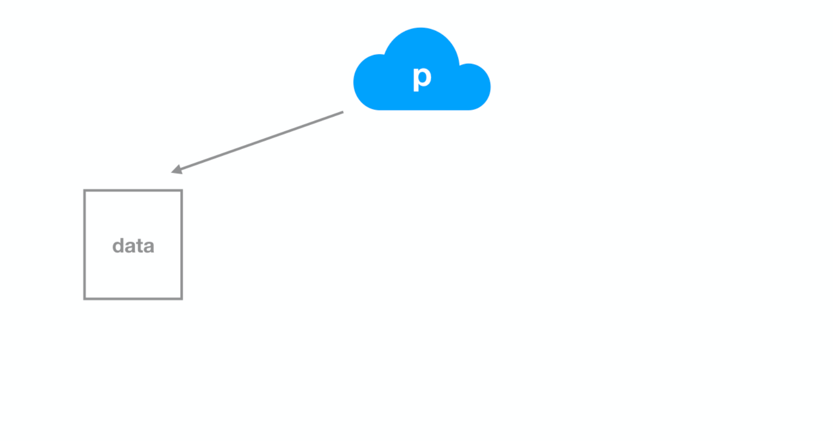
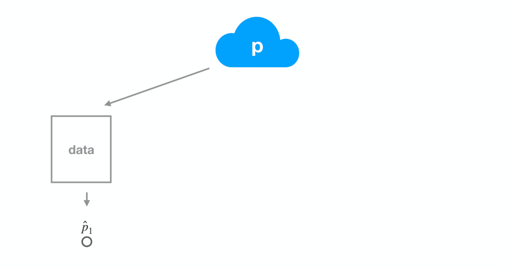
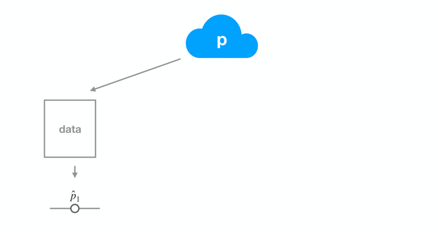
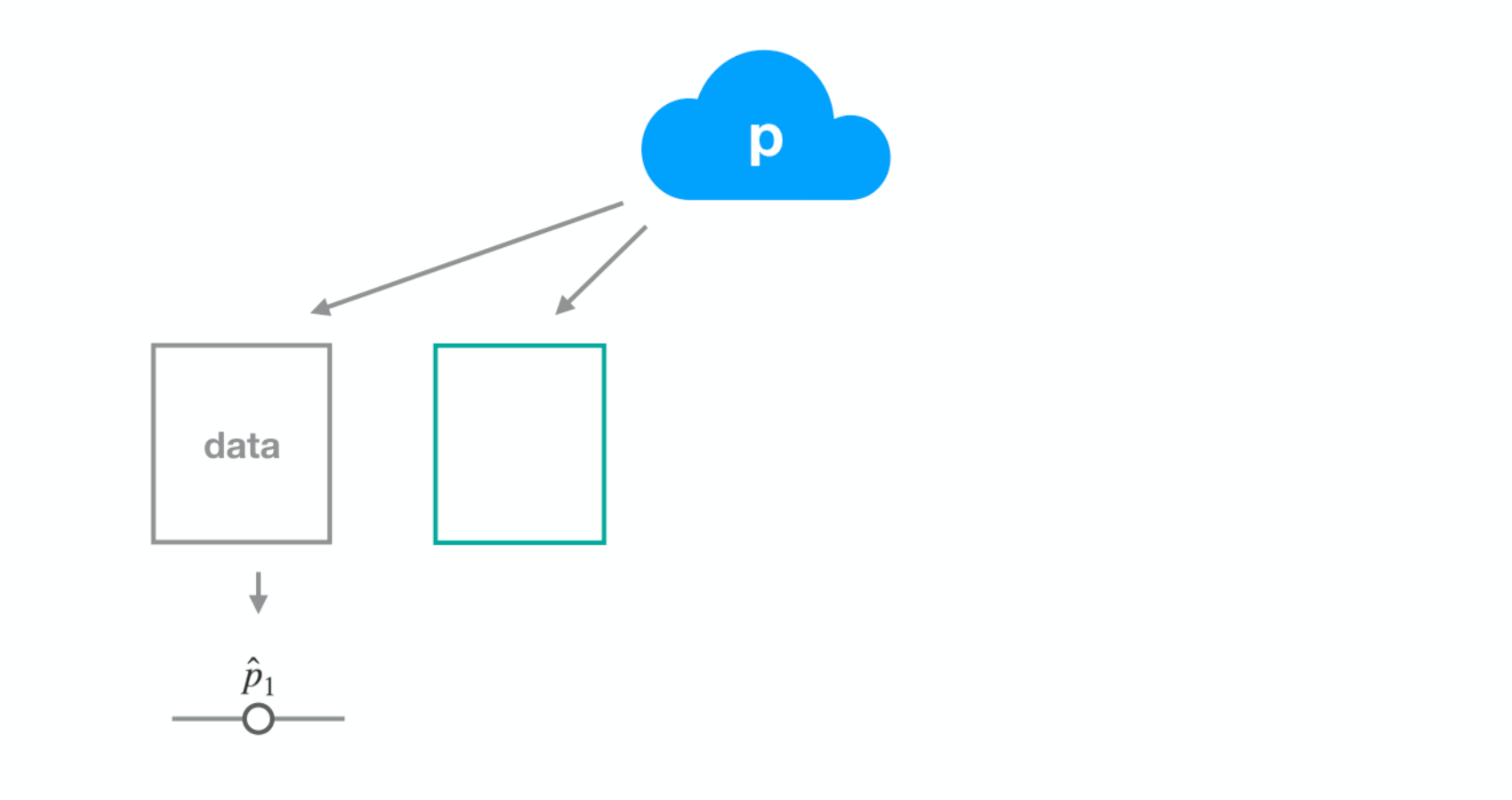
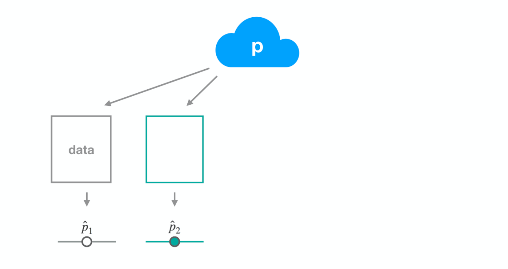
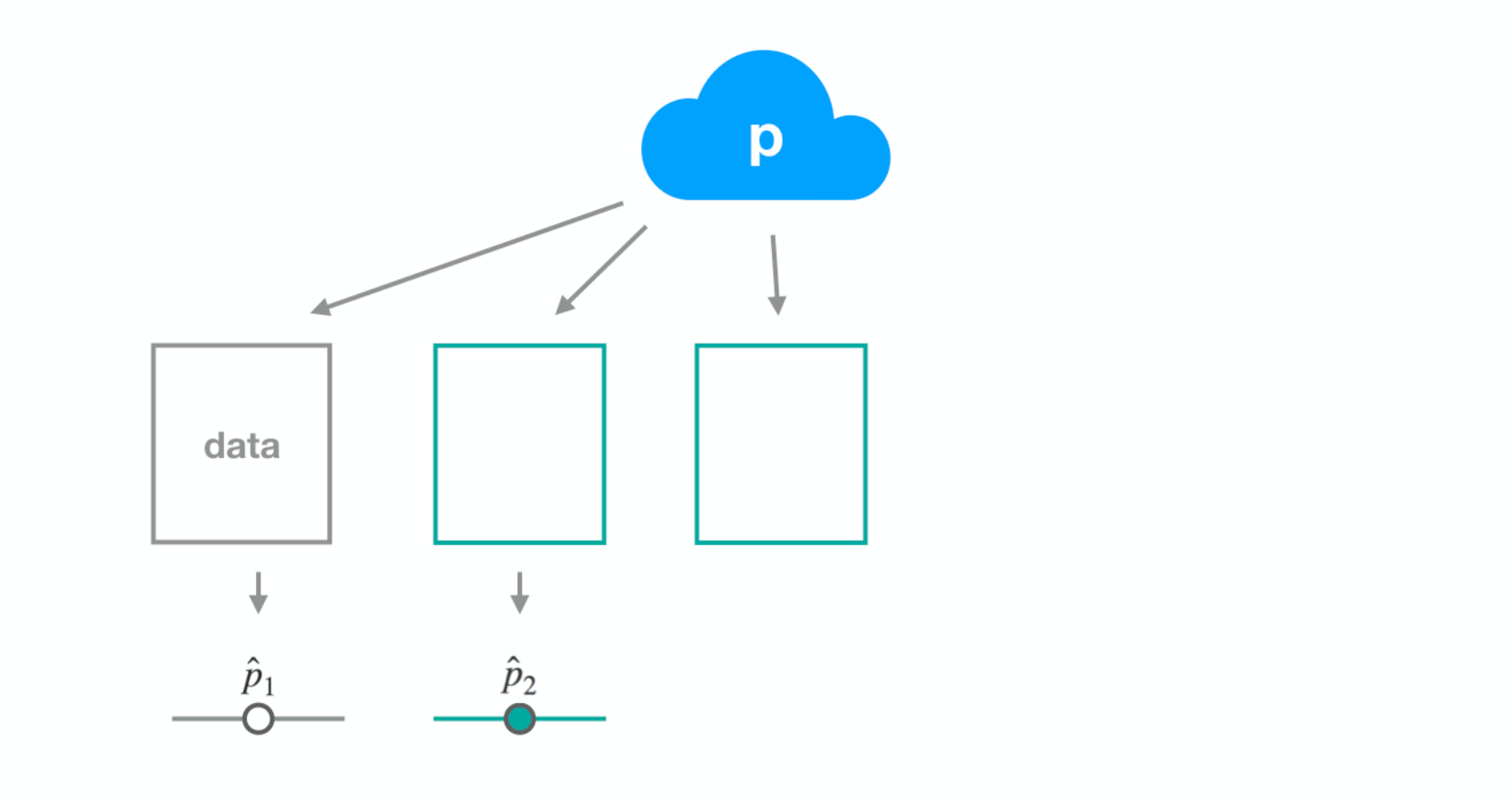
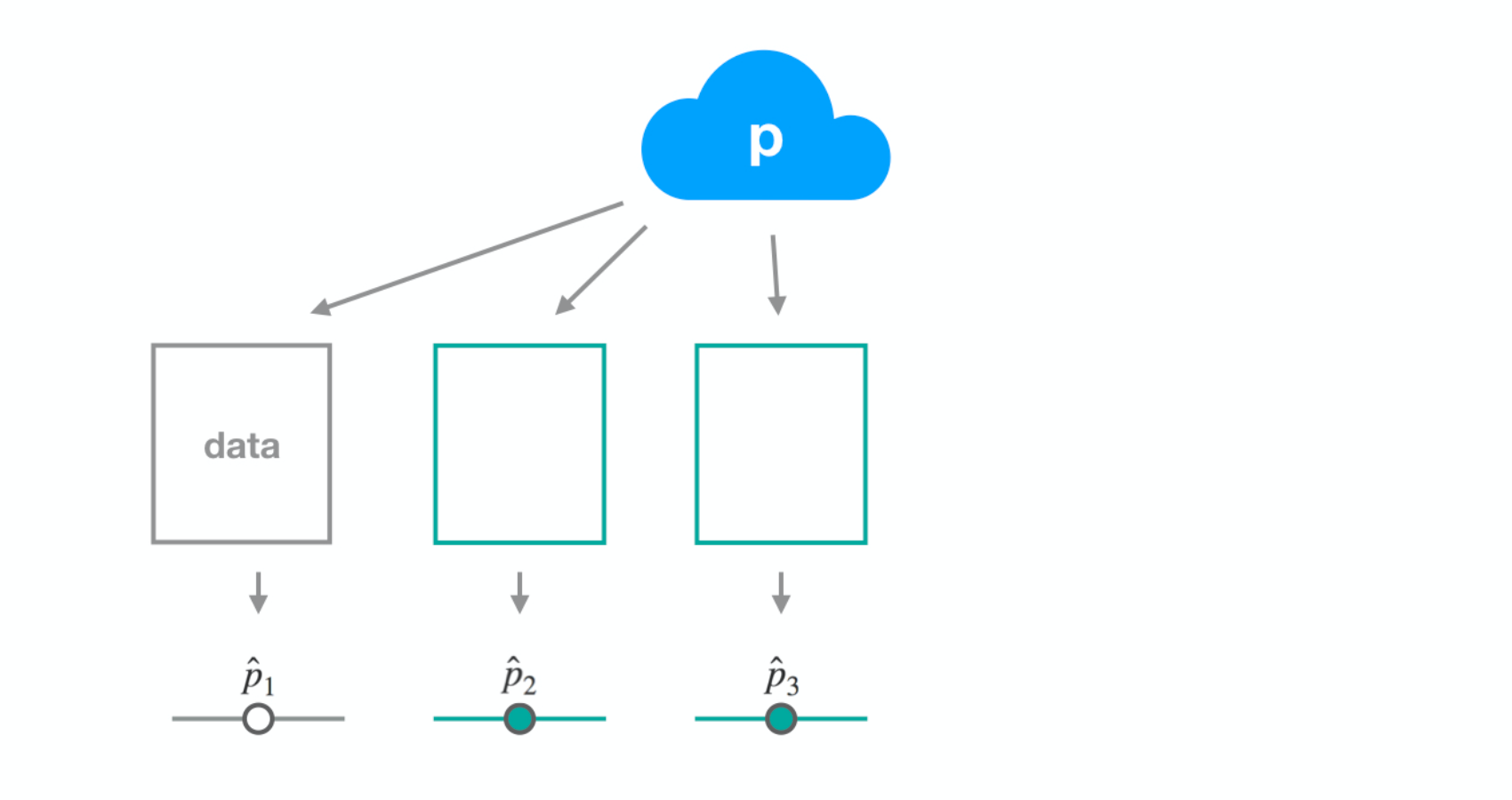
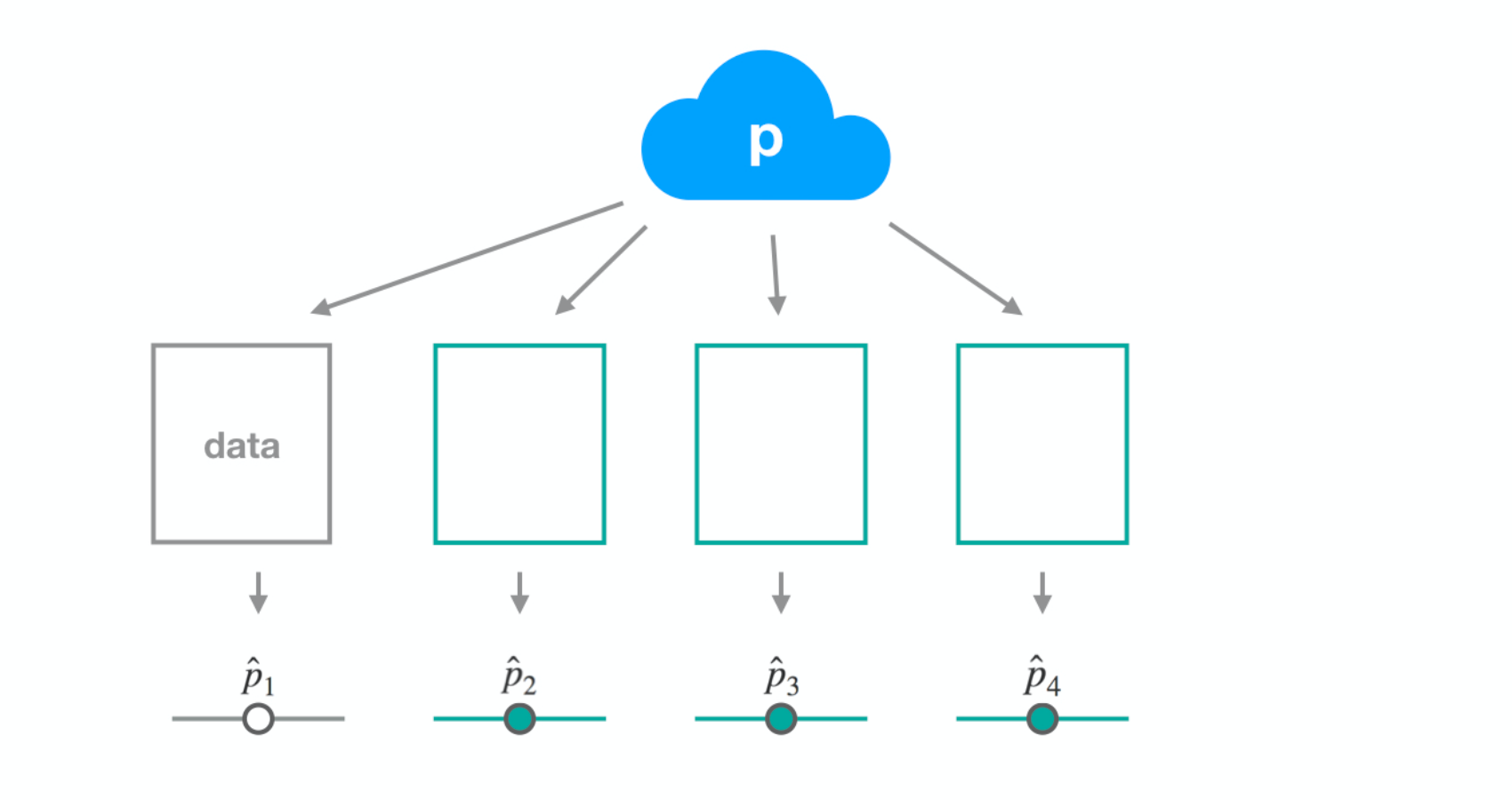
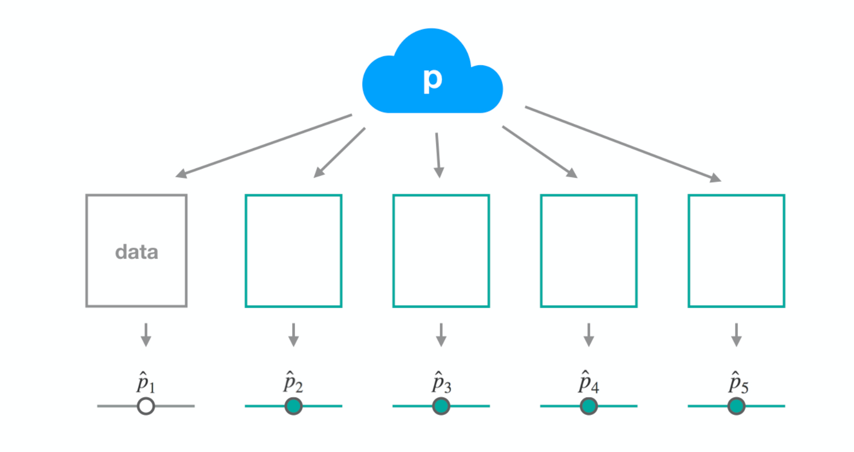
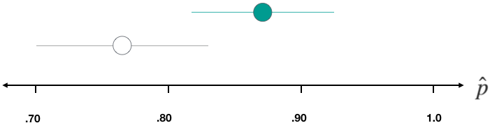
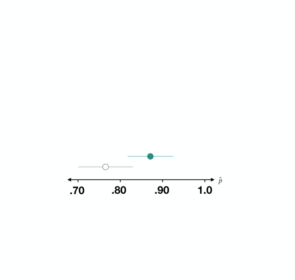
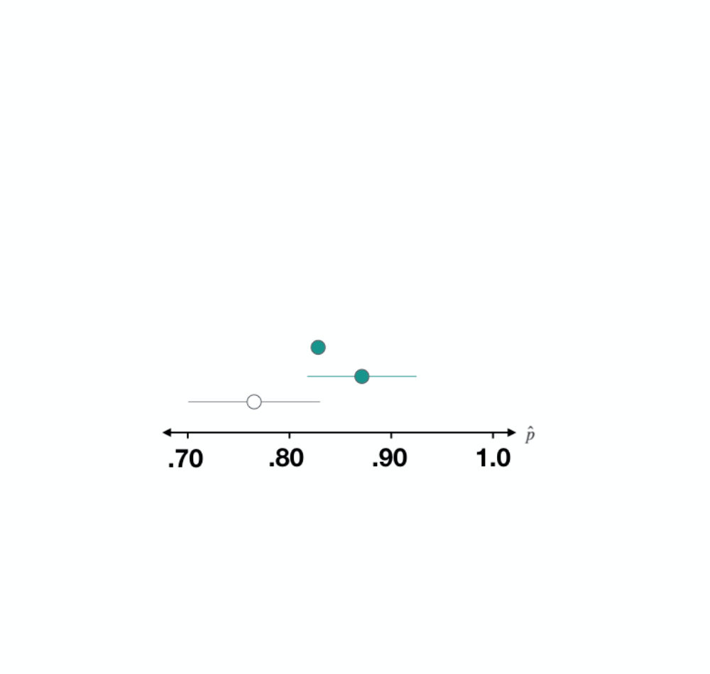
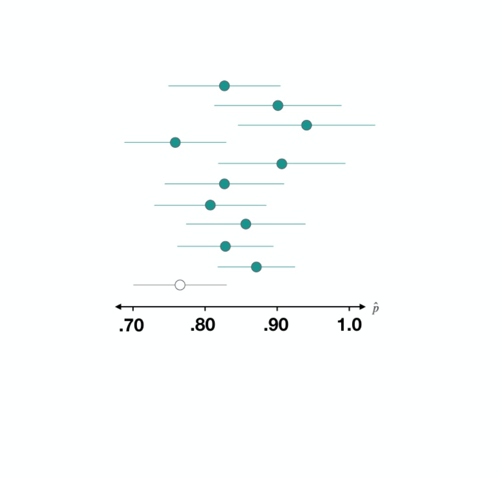
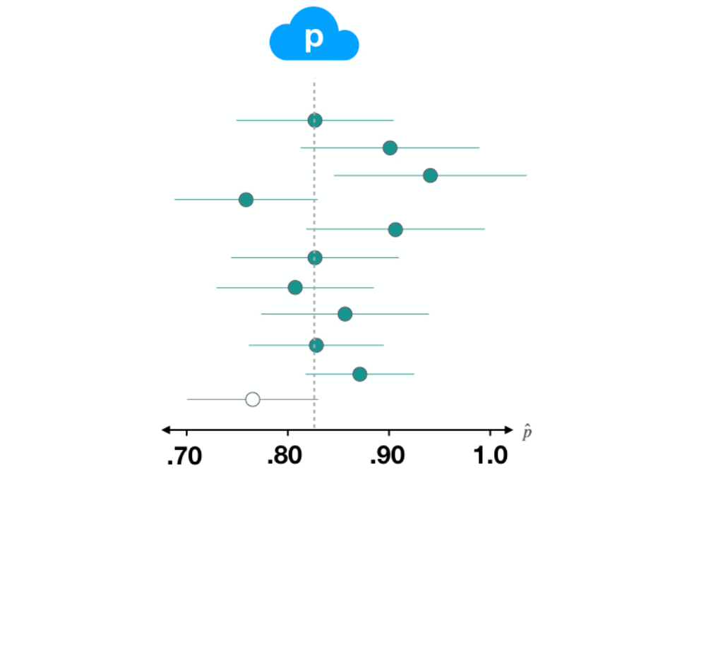
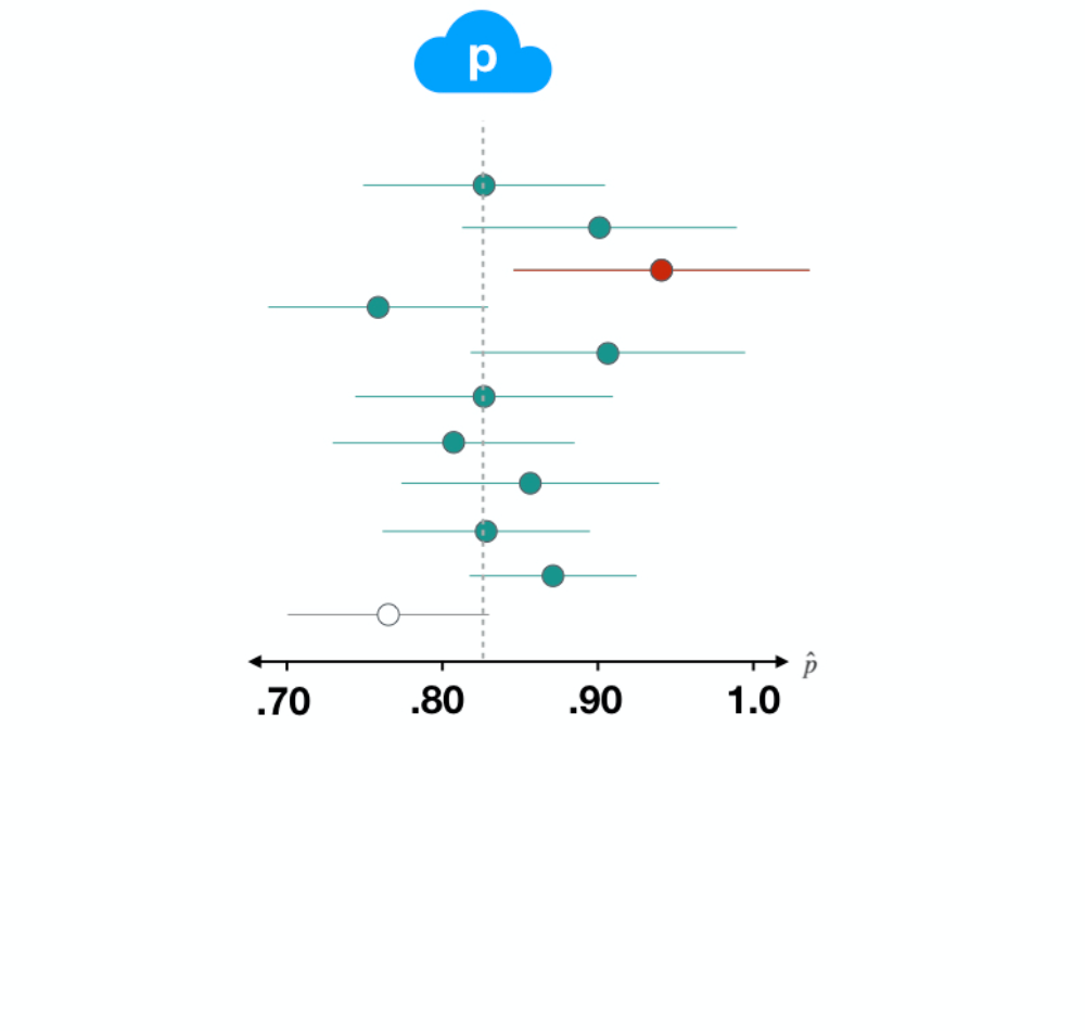
Vad menar vi med konfident?
ds1 <- filter(gss, year == 2016)p_hat <- ds1 %>% summarize(mean(happy == "HAPPY")) %>% pull()SE <- ds1 %>% specify(response = happy, success = "HAPPY") %>% generate(reps = 500, type = "bootstrap") %>% calculate(stat = "prop") %>% summarize(sd(stat)) %>% pull()c(p_hat - 2 * SE, p_hat + 2 * SE)
0.7073114 0.8393553


ds2 <- filter(gss, year == 2014)p_hat <- ds1 %>% summarize(mean(happy == "HAPPY")) %>% pull()SE <- ds1 %>% specify(response = happy, success = "HAPPY") %>% generate(reps = 500, type = "bootstrap") %>% calculate(stat = "prop") %>% summarize(sd(stat)) %>% pull()c(p_hat - 2 * SE, p_hat + 2 * SE)
0.8348831 0.9384503

ds3 <- filter(gss, year == 2012)p_hat <- ds1 %>% summarize(mean(happy == "HAPPY")) %>% pull()SE <- ds1 %>% specify(response = happy, success = "HAPPY") %>% generate(reps = 500, type = "bootstrap") %>% calculate(stat = "prop") %>% summarize(sd(stat)) %>% pull()c(p_hat - 2 * SE, p_hat + 2 * SE)
0.7626359 0.8906974

ds3 <- filter(gss, year == 2012) p_hat <- ds3 %>% summarize(mean(happy == "HAPPY")) %>% pull() SE <- ds3 %>% specify(response = happy, success = "HAPPY") %>% generate(reps = 500, type = "bootstrap") %>% calculate(stat = "prop") %>% summarize(sd(stat)) %>% pull()c(p_hat - 2 * SE, p_hat + 2 * SE)
0.7626359 0.8906974

ds3 <- filter(gss, year == 2012) p_hat <- ds3 %>% summarize(mean(happy == "HAPPY")) %>% pull() SE <- ds3 %>% specify(response = happy, success = "HAPPY") %>% generate(reps = 500, type = "bootstrap") %>% calculate(stat = "prop") %>% summarize(sd(stat)) %>% pull()c(p_hat - 2 * SE, p_hat + 2 * SE)
0.7626359 0.8906974

ds3 <- filter(gss, year == 2012) p_hat <- ds3 %>% summarize(mean(happy == "HAPPY")) %>% pull() SE <- ds3 %>% specify(response = happy, success = "HAPPY") %>% generate(reps = 500, type = "bootstrap") %>% calculate(stat = "prop") %>% summarize(sd(stat)) %>% pull()c(p_hat - 2 * SE, p_hat + 2 * SE)
0.7626359 0.8906974

ds3 <- filter(gss, year == 2012) p_hat <- ds3 %>% summarize(mean(happy == "HAPPY")) %>% pull() SE <- ds3 %>% specify(response = happy, success = "HAPPY") %>% generate(reps = 500, type = "bootstrap") %>% calculate(stat = "prop") %>% summarize(sd(stat)) %>% pull()c(p_hat - 2 * SE, p_hat + 2 * SE)
0.7626359 0.8906974

ds3 <- filter(gss, year == 2012) p_hat <- ds3 %>% summarize(mean(happy == "HAPPY")) %>% pull() SE <- ds3 %>% specify(response = happy, success = "HAPPY") %>% generate(reps = 500, type = "bootstrap") %>% calculate(stat = "prop") %>% summarize(sd(stat)) %>% pull()c(p_hat - 2 * SE, p_hat + 2 * SE)
0.7626359 0.8906974

Tolkning: "Vi är 95 % säkra på att den sanna andelen amerikaner som är lyckliga ligger mellan 0,705 och 0,841."
Intervallets bredd påverkas av
npInferens för kategoriska data i R