ไม่เจ็บปวด ไม่ก้าวหน้า

GARCH Models in R

Kris Boudt

Professor of finance and econometrics

โมเดล GARCH-in-mean

วัดปริมาณความสัมพันธ์ระหว่างความเสี่ยงและผลตอบแทน
ความเสี่ยง: $\sigma^2_t$. ผลตอบแทน: $\mu_t$.
โมเดล GARCH-in-mean:

$$ \mu_{t} = \mu + \lambda \sigma^2_{t} $$

$\lambda > 0$ คือพารามิเตอร์ความเสี่ยง/ผลตอบแทน บ่งชี้การเพิ่มขึ้นของผลตอบแทนที่คาดหวังต่อหนึ่งหน่วยความเสี่ยงของ Variance

ทำอย่างไร?

เปลี่ยนอาร์กิวเมนต์ mean.model ใน ugarchspec() จาก list(armaOrder = c(0, 0)) เป็น list(armaOrder = c(0, 0), archm = TRUE, archpow = 2):

garchspec <- ugarchspec(
              mean.model = list(armaOrder = c(0, 0)),
              variance.model = list(model = "gjrGARCH"),
              distribution.model = "sstd")

garchspec <- ugarchspec(
               mean.model = list(armaOrder = c(0, 0), archm = TRUE, archpow = 2),
               variance.model = list(model = "gjrGARCH"),
               distribution.model = "sstd")

การประยุกต์ใช้กับผลตอบแทนรายวันของ S&P 500

การประมาณค่า

garchfit <- ugarchfit(data = sp500ret, spec = garchspec)

ตรวจสอบค่าสัมประสิทธิ์ที่ประมาณได้สำหรับ Mean

round(coef(garchfit)[1:2], 4)

    mu  archm 
0.0002 1.9950

ค่าเฉลี่ยผลตอบแทนที่พยากรณ์ได้

$$ \hat{\mu}_{t} = 0.0002 + 1.9950 \hat{\sigma}^2_{t} $$

กราฟอนุกรมเวลาของผลตอบแทนที่พยากรณ์

พล็อตกราฟใน R
```
plot(fitted(garchfit))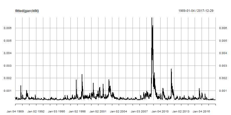
```

ผลตอบแทนวันนี้พยากรณ์ผลตอบแทนวันพรุ่งนี้

GARCH-in-mean ใช้ทฤษฎีทางการเงินเรื่องความสัมพันธ์ระหว่างความเสี่ยงและผลตอบแทนเพื่อสร้างโมเดล Conditional Mean
ต่อมาจะใช้ทฤษฎีทางสถิติเพื่อสร้างโมเดล Mean ที่อาศัยความสัมพันธ์ระหว่างผลตอบแทนวันนี้กับวันพรุ่งนี้
โมเดลที่นิยมที่สุดคือโมเดล AR(1):
- AR(1) ย่อมาจาก Autoregressive Model of Order 1
- ใช้ส่วนเบี่ยงเบนของผลตอบแทนจากค่าเฉลี่ยระยะยาว $\mu$ เพื่อพยากรณ์ผลตอบแทนถัดไป:

$$ \mu_{t} = \mu + \rho(R_{t-1} - \mu) $$

สัมประสิทธิ์ Autoregressive ที่เป็นบวก

$$ \mu_{t} = \mu + \rho(R_{t-1} - \mu) $$

$\rho > 0$:
- ผลตอบแทนที่สูง (ต่ำ) กว่าค่าเฉลี่ยจะตามมาด้วยผลตอบแทนที่สูง (ต่ำ) กว่าค่าเฉลี่ยเช่นกัน
- คำอธิบายที่เป็นไปได้: ตลาดตอบสนองต่อข่าวสารไม่เพียงพอ จึงเกิดโมเมนตัมในผลตอบแทน
$|\rho|<1$: Mean Reversion: ส่วนเบี่ยงเบนของ $R_t$ จาก $\mu$ เป็นเพียงชั่วคราว

สัมประสิทธิ์ Autoregressive ที่เป็นลบ

$$ \mu_{t} = \mu + \rho(R_{t-1} - \mu) $$

$\rho < 0$:
- ผลตอบแทนที่สูง (ต่ำ) กว่าค่าเฉลี่ยจะตามมาด้วยผลตอบแทนที่ต่ำ (สูง) กว่าค่าเฉลี่ย
- คำอธิบายที่เป็นไปได้: ตลาดตอบสนองต่อข่าวสารมากเกินไป จึงเกิดการกลับตัวในผลตอบแทน

การประยุกต์ใช้กับผลตอบแทนรายวันของ S&P 500

การกำหนดสเปกและการประมาณค่า AR(1)-GJR GARCH ด้วยการแจกแจงแบบ sst

garchspec <- ugarchspec( 
          mean.model = list(armaOrder = c(1, 0)),
          variance.model = list(model = "gjrGARCH"),
          distribution.model = "sstd")
garchfit <- ugarchfit(data = sp500ret, spec = garchspec)

ค่าประมาณของโมเดล AR(1)

round(coef(garchfit)[1:2], 4)

     mu     ar1     
 0.0003 -0.0292

โมเดล MA(1) และ ARMA(1,1)

โมเดล Moving Average อันดับ 1 ใช้ส่วนเบี่ยงเบนของผลตอบแทนจาก Conditional Mean:

$$ \mu_{t} = \mu + \theta(R_{t-1} - \mu_{t-1}) $$

ARMA(1,1) รวม AR(1) และ MA(1) เข้าด้วยกัน:

$$ \mu_{t} = \mu + \rho(R_{t-1} - \mu) + \theta(R_{t-1} - \mu_{t-1}) $$

ทำอย่างไร?

MA(1)

garchspec <- ugarchspec( 
          mean.model = list(armaOrder = c(0, 1)),
          variance.model = list(model = "gjrGARCH"),
          distribution.model = "sstd")

ARMA(1, 1)

garchspec <- ugarchspec( 
          mean.model = list(armaOrder = c(1, 1)),
          variance.model = list(model = "gjrGARCH"),
          distribution.model = "sstd")

ถึงคิวของคุณแล้ว — ลองเปลี่ยนอาร์กิวเมนต์ mean.model

GARCH Models in R