Вибір кількості компонентів

Багатовимірні ймовірнісні розподіли в R

Surajit Ray

Professor, University of Glasgow

Підсумок об'єкта princomp

summary(cars.pca)

Importance of components:
                       Comp.1 Comp.2 Comp.3 Comp.4 Comp.5 Comp.6 Comp.7 Comp.8  Comp.9
Standard deviation      2.378  1.443  0.710 0.5148 0.4280 0.3518 0.3241 0.2419 0.14896
Proportion of Variance  0.628  0.231  0.056 0.0294 0.0204 0.0138 0.0117 0.0065 0.00247
Cumulative Proportion   0.628  0.860  0.916 0.9453 0.9656 0.9794 0.9910 0.9975 1.00000

Використання графіка осипу

Метод 1

Частка поясненої варіації

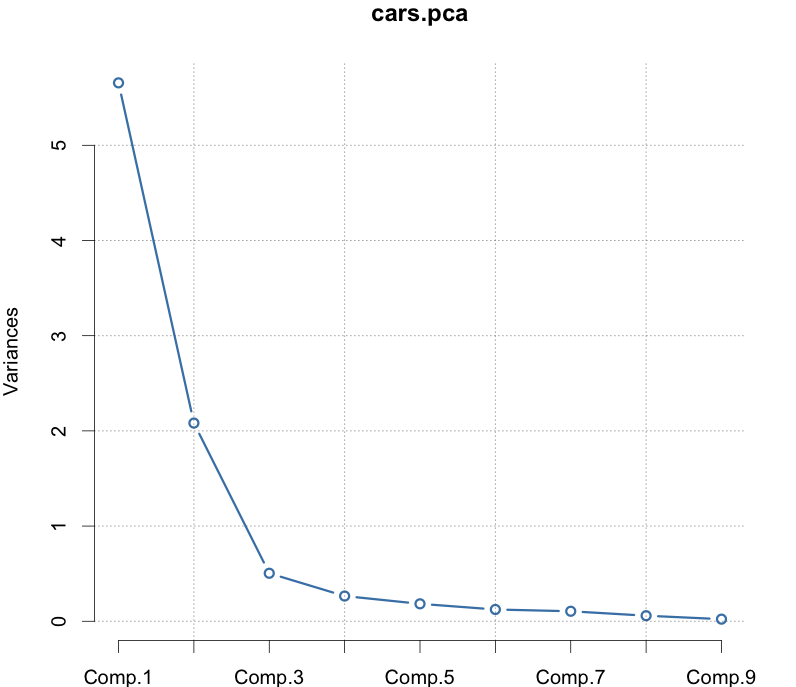
screeplot(cars.pca, type = "lines")

Вибір на основі

крутизни кривої
після якої йде плоска ділянка

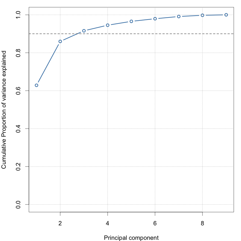
Пояснена кумулятивна дисперсія

Метод 2

Кумулятивна варіація
Пояснити задане значення

summary(cars.pca)

Importance of components:
                      Comp.1 Comp.2 Comp.3 Comp.4 Comp.5 Comp.6 Comp.7 Comp.8  Comp.9
Standard deviation     2.378  1.443  0.710 0.5148 0.4280 0.3518 0.3241 0.2419 0.14896
Proportion of Variance 0.628  0.231  0.056 0.0294 0.0204 0.0138 0.0117 0.0065 0.00247
Cumulative Proportion  0.628  0.860  0.916 0.9453 0.9656 0.9794 0.9910 0.9975 1.00000

Обчислення кумулятивної пропорційної дисперсії

Кумулятивна частка

# Variance explained
pc.var <- cars.pca$sdev^2

# Proportion of variation
pc.pvar <- pc.var / sum(pc.var)

# Cumulative proportion
plot(cumsum(pc.pvar), type = 'b')

abline(h = 0.9, lty = 2)

Обчислення кумулятивної пропорційної дисперсії

Кумулятивна частка

# Variance explained
pc.var <- cars.pca$sdev^2

# Proportion of variation
pc.pvar <- pc.var / sum(pc.var)

# Cumulative proportion
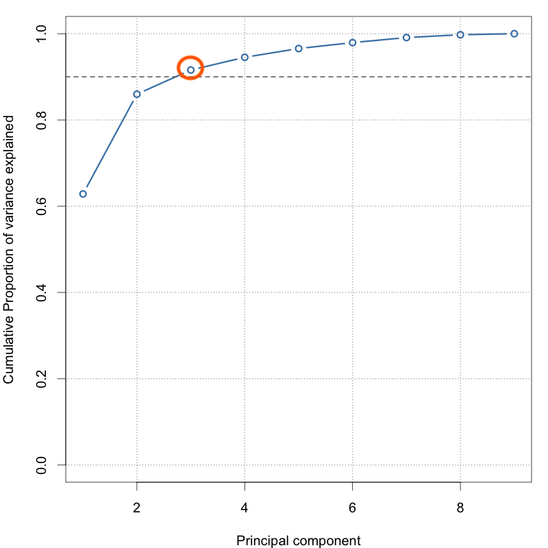
plot(cumsum(pc.pvar), type = 'b')

abline(h = 0.9, lty = 2)

3 ГК пояснюють 90 відсотків варіації

Давайте потренуємось, використовуючи ці методи!

Багатовимірні ймовірнісні розподіли в R