인덱스 상관관계 & Excel 내보내기

Python으로 시계열 데이터 다루기

Stefan Jansen

Founder & Lead Data Scientist at Applied Artificial Intelligence

인덱스 추가 분석

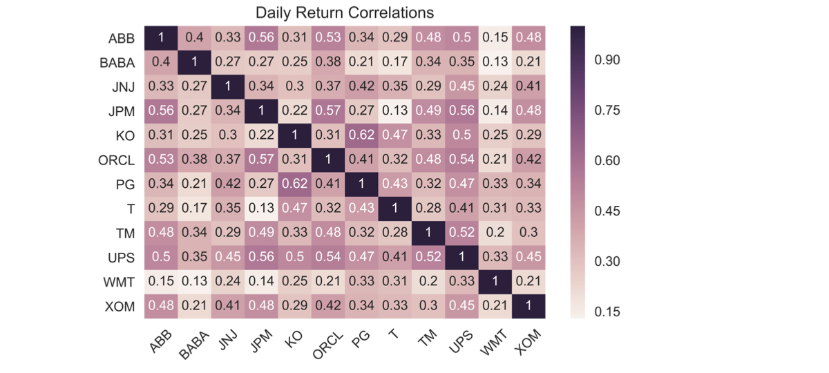
일별 수익률 상관관계:
모든 구성 종목 간 계산
결과를 히트맵으로 시각화
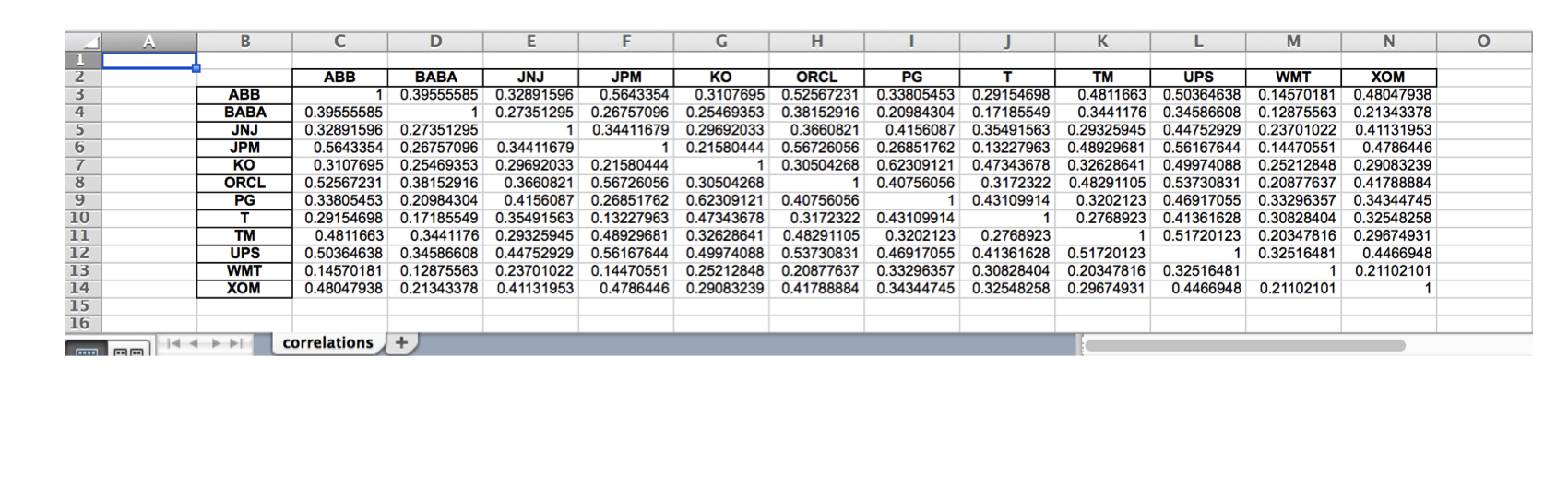
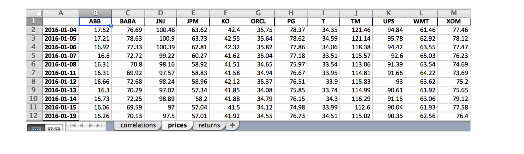
.xls 및 .xlsx 형식으로 Excel에 저장:
단일 워크시트
다중 워크시트

인덱스 구성 종목 - 가격 데이터

data = DataReader(tickers, 'google', start='2016', end='2017')['Close']

data.info()

DatetimeIndex: 252 entries, 2016-01-04 to 2016-12-30
Data columns (total 12 columns):
ABB     252 non-null float64
BABA    252 non-null float64
JNJ     252 non-null float64
JPM     252 non-null float64
KO      252 non-null float64
ORCL    252 non-null float64
PG      252 non-null float64
T       252 non-null float64
TM      252 non-null float64
UPS     252 non-null float64
WMT     252 non-null float64
XOM     252 non-null float64

인덱스 구성 종목: 수익률 상관관계

daily_returns = data.pct_change()

correlations = daily_returns.corr()

ABB  BABA  JNJ  JPM   KO  ORCL   PG    T   TM  UPS  WMT  XOM
ABB  1.00  0.40 0.33 0.56 0.31  0.53 0.34 0.29 0.48 0.50 0.15 0.48
BABA 0.40  1.00 0.27 0.27 0.25  0.38 0.21 0.17 0.34 0.35 0.13 0.21
JNJ  0.33  0.27 1.00 0.34 0.30  0.37 0.42 0.35 0.29 0.45 0.24 0.41
JPM  0.56  0.27 0.34 1.00 0.22  0.57 0.27 0.13 0.49 0.56 0.14 0.48
KO   0.31  0.25 0.30 0.22 1.00  0.31 0.62 0.47 0.33 0.50 0.25 0.29
ORCL 0.53  0.38 0.37 0.57 0.31  1.00 0.41 0.32 0.48 0.54 0.21 0.42
PG   0.34  0.21 0.42 0.27 0.62  0.41 1.00 0.43 0.32 0.47 0.33 0.34
T    0.29  0.17 0.35 0.13 0.47  0.32 0.43 1.00 0.28 0.41 0.31 0.33
TM   0.48  0.34 0.29 0.49 0.33  0.48 0.32 0.28 1.00 0.52 0.20 0.30
UPS  0.50  0.35 0.45 0.56 0.50  0.54 0.47 0.41 0.52 1.00 0.33 0.45
WMT  0.15  0.13 0.24 0.14 0.25  0.21 0.33 0.31 0.20 0.33 1.00 0.21
XOM  0.48  0.21 0.41 0.48 0.29  0.42 0.34 0.33 0.30 0.45 0.21 1.00

인덱스 구성 종목: 수익률 상관관계

sns.heatmap(correlations, annot=True)
plt.xticks(rotation=45)
plt.title('Daily Return Correlations')

ch4_4_v2 - Index Correlation & Saving Results to Excel.010.png

단일 Excel 워크시트에 저장하기

correlations.to_excel(excel_writer= 'correlations.xls',
                      sheet_name='correlations',
                      startrow=1,
                      startcol=1)

ch4_4_v2 - Index Correlation & Saving Results to Excel.012.png

다중 Excel 워크시트에 저장하기

data.index = data.index.date # Keep only date component

with pd.ExcelWriter('stock_data.xlsx') as writer:

    corr.to_excel(excel_writer=writer, sheet_name='correlations')

    data.to_excel(excel_writer=writer, sheet_name='prices')

    data.pct_change().to_excel(writer, sheet_name='returns')

ch4_4_v2 - Index Correlation & Saving Results to Excel.015.png

연습해 봅시다!

Python으로 시계열 데이터 다루기