Sonuçların görselleştirilmesi

R ile Bioconductor kullanarak RNA-Seq

Mary Piper

Bioinformatics Consultant and Trainer

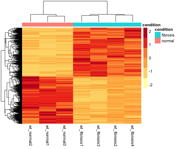
Sonuçları görselleştirme - Ekspresyon ısı haritası

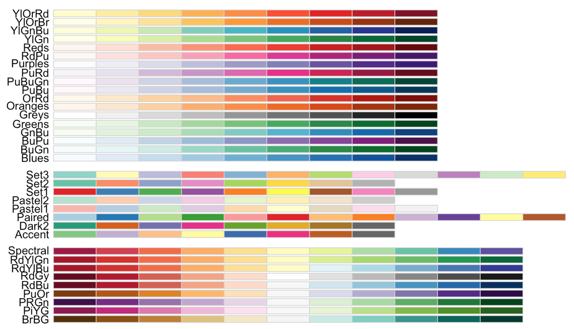
# Önemli genler için normalize edilmiş sayımları alt kümele 
sig_norm_counts_wt <- normalized_counts_wt[wt_res_sig$ensgene, ]

# RColorBrewer'dan bir renk paleti seç
library(RColorBrewer) 
heat_colors <- brewer.pal(6, "YlOrRd")

display.brewer.all()

renk paletleri

Sonuçları görselleştirme - Ekspresyon ısı haritası

# pheatmap'i çalıştır
pheatmap(sig_norm_counts_wt, 
         color = heat_colors, 
         cluster_rows = T, 
         show_rownames = F,
         annotation = select(wt_metadata, condition), 
         scale = "row")

ekspresyon ısı haritası

Sonuçları görselleştirme - Volkan grafiği

# padj değerlerinin 0.05'ten küçük olup olmadığını gösteren mantıksal bir vektör elde et 
wt_res_all <- wt_res_all %>%
              rownames_to_column(var = "ensgene") %>%
              mutate(threshold = padj < 0.05)

# Volkan grafiği
ggplot(wt_res_all) +
        geom_point(aes(x = log2FoldChange, y = -log10(padj), 
                   color = threshold)) +
        xlab("log2 fold change") + 
        ylab("-log10 adjusted p-value") +
        theme(legend.position = "none",
              plot.title = element_text(size = rel(1.5), hjust = 0.5),
              axis.title = element_text(size = rel(1.25)))

ggplot(wt_res_all) +
        geom_point(aes(x = log2FoldChange, y = -log10(padj), color = threshold)) +
        xlab("log2 fold change") + 
        ylab("-log10 adjusted p-value") +
        ylim=c(0, 15) +
        theme(legend.position = "none",
              plot.title = element_text(size = rel(1.5), hjust = 0.5),
              axis.title = element_text(size = rel(1.25)))

yakınlaştırılmış volkan grafiği

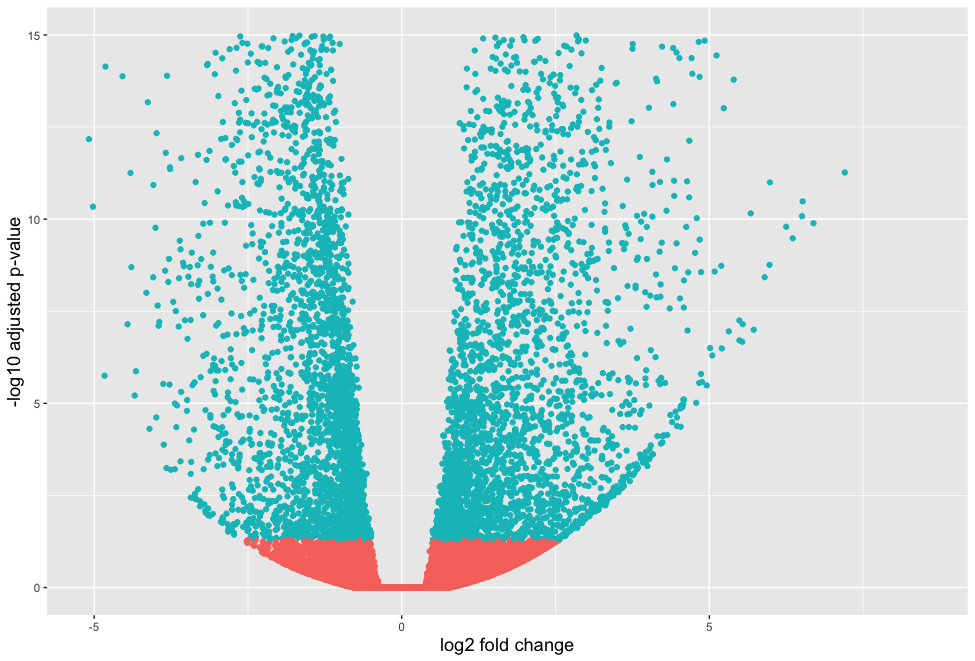
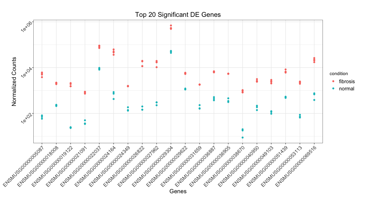
Sonuçları görselleştirme - Ekspresyon grafiği

Önemli sonuçlar:

önemli sonuçlar

Önemli genler için normalize edilmiş sayımlar:

önemli normalize sayımlar

Sonuçları görselleştirme - Ekspresyon grafiği

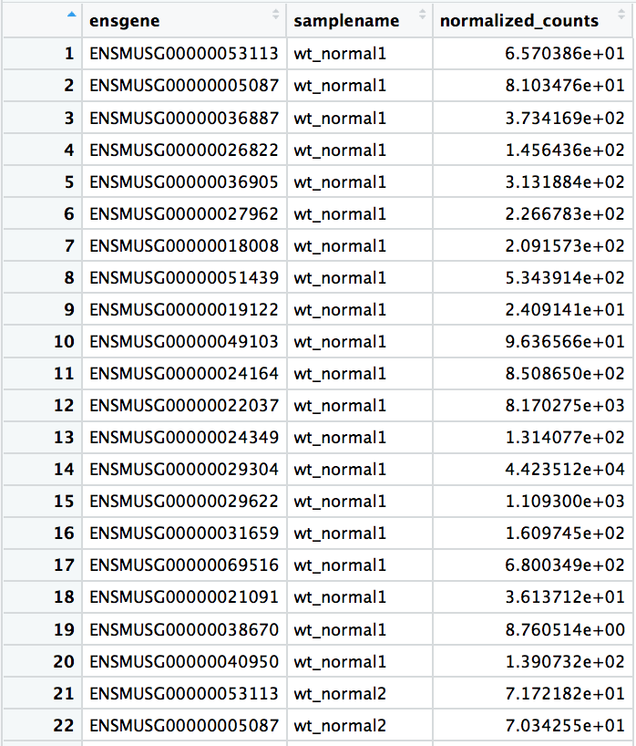
top_20 <- data.frame(sig_norm_counts_wt)[1:20, ] %>%
        rownames_to_column(var = "ensgene")

top_20 <- gather(top_20, key = "samplename", value = "normalized_counts", 2:8)

toplanan normalize sayımlar

Sonuçları görselleştirme - Ekspresyon grafiği

top_20 <- inner_join(top_20,
                     rownames_to_column(wt_metadata, var = "samplename"),
                     by = "samplename")

ggplot(top_20) +
        geom_point(aes(x = ensgene, y = normalized_counts, color = condition)) +
        scale_y_log10() +
        xlab("Genler") +
        ylab("Normalize Edilmiş Sayımlar") +
        ggtitle("En Önemli 20 DE Gen") +
        theme_bw() +
        theme(axis.text.x = element_text(angle = 45, hjust = 1)) +
        theme(plot.title = element_text(hjust = 0.5))

ilk 20 ekspresyon grafiği

Hadi pratik yapalım!

R ile Bioconductor kullanarak RNA-Seq