為什麼需要邏輯斯迴歸

R 迴歸入門

Richie Cotton

Data Evangelist at DataCamp

銀行流失資料集

has_churned	time_since_first_purchase	time_since_last_purchase
0	0.3993247	-0.5158691
1	-0.4297957	0.6780654
0	3.7383122	0.4082544
0	0.6032289	-0.6990435
...	...	...
response	length of relationship	recency of activity

¹ https://www.rdocumentation.org/packages/bayesQR/topics/Churn

流失 vs. 最近性：線性模型

mdl_churn_vs_recency_lm <- lm(has_churned ~ time_since_last_purchase, data = churn)

Call:
lm(formula = has_churned ~ time_since_last_purchase, data = churn)

Coefficients:
             (Intercept)  time_since_last_purchase  
                 0.49078                   0.06378

coeffs <- coefficients(mdl_churn_vs_recency_lm)
intercept <- coeffs[1]
slope <- coeffs[2]

視覺化線性模型

ggplot(
  churn, 
  aes(time_since_last_purchase, has_churned)
) +
  geom_point() +
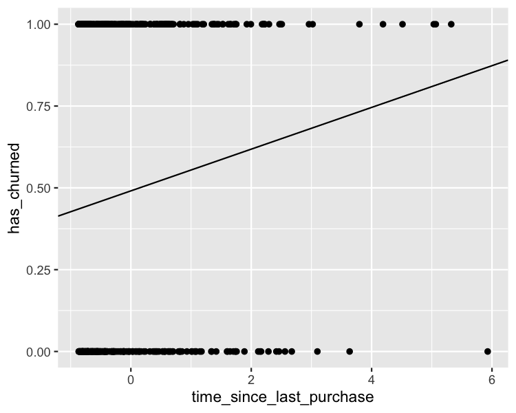
  geom_abline(intercept = intercept, slope = slope)

「預測」是流失機率，而不是流失數量。

一張散佈圖，顯示顧客是否流失與距上次購買時間的關係。所有點都在 y=0 或 y=1 的直線上。線性趨勢線顯示，距上次購買時間越長，流失機率越高。

拉遠視角

ggplot(
  churn, 
  aes(days_since_last_purchase, has_churned)
) +
  geom_point() +
  geom_abline(intercept = intercept, slope = slope) +
  xlim(-10, 10) +
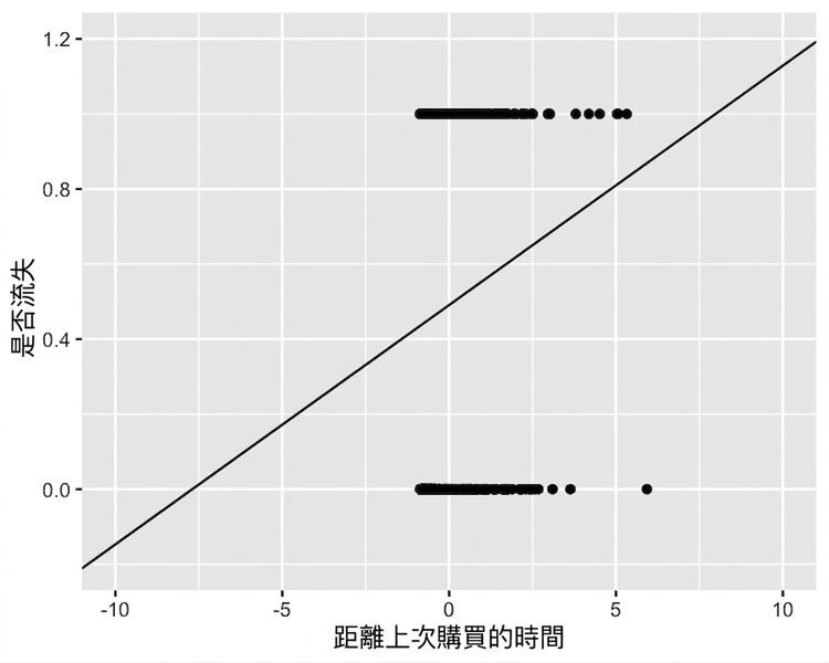
  ylim(-0.2, 1.2)

與前一張相同的散佈圖，但座標軸縮小視角。可見趨勢線延伸到 y 小於 0 且大於 1 的範圍，這在機率上是不可能的。

什麼是邏輯斯迴歸？

一種廣義線性模型。
當反應變數為邏輯型時使用。
反應遵循邏輯（S 形）曲線。

使用 glm() 的線性迴歸

glm(has_churned ~ time_since_last_purchase, data = churn, family = gaussian)

Call:  glm(formula = has_churned ~ time_since_last_purchase, family = gaussian, 
    data = churn)

Coefficients:
             (Intercept)  time_since_last_purchase  
                 0.49078                   0.06378  

Degrees of Freedom: 399 Total (i.e. Null);  398 Residual
Null Deviance:        100 
Residual Deviance: 98.02     AIC: 578.7

邏輯斯迴歸：glm() 與二項分佈家族

mdl_recency_glm <- glm(has_churned ~ time_since_last_purchase, data = churn, family = binomial)

Call:  glm(formula = has_churned ~ time_since_last_purchase, family = binomial, 
    data = churn)

Coefficients:
             (Intercept)  time_since_last_purchase  
                -0.03502                   0.26921  

Degrees of Freedom: 399 Total (i.e. Null);  398 Residual
Null Deviance:        554.5 
Residual Deviance: 546.4     AIC: 550.4

視覺化邏輯斯模型

ggplot(
  churn, 
  aes(time_since_last_purchase, has_churned)
) +
  geom_point() +
  geom_abline(
    intercept = intercept, slope = slope
  ) +
  geom_smooth(
    method = "glm", 
    se = FALSE, 
    method.args = list(family = binomial)
  )

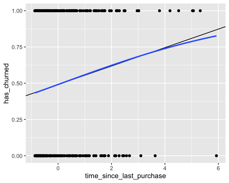
一張散佈圖，顯示顧客是否流失與距上次購買時間的關係。線性與邏輯斯趨勢線皆顯示，時間越長流失機率越高。除在高「距上次購買時間」區域外，兩條線大致相近。

拉遠視角

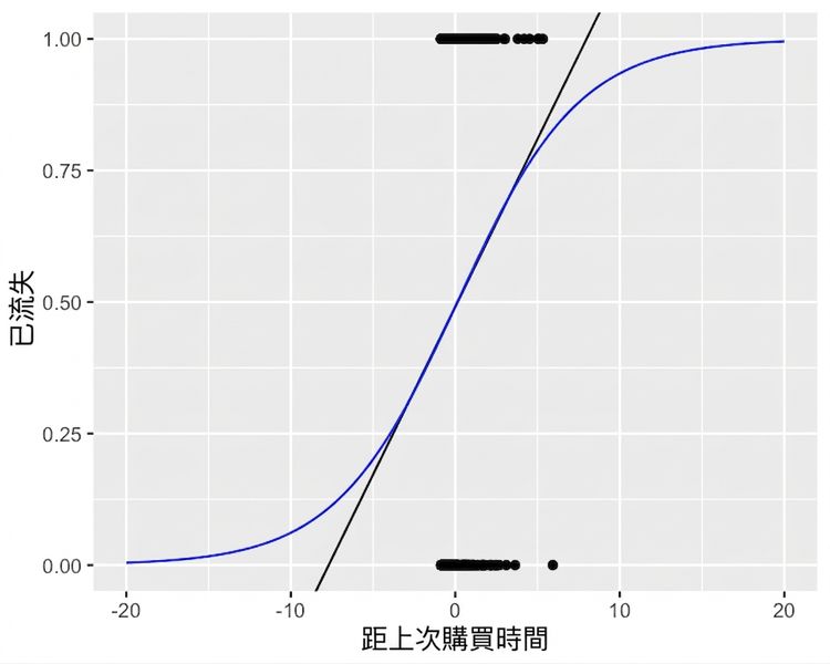
與前一張相同的散佈圖，含兩條趨勢線。座標軸拉遠後可見，邏輯斯趨勢線始終維持在 0 到 1 的流失範圍內。

一起來練習吧！

R 迴歸入門