實驗設計中的共變數調整

Python 的實驗設計

James Chapman

Curriculum Manager, DataCamp

共變數入門

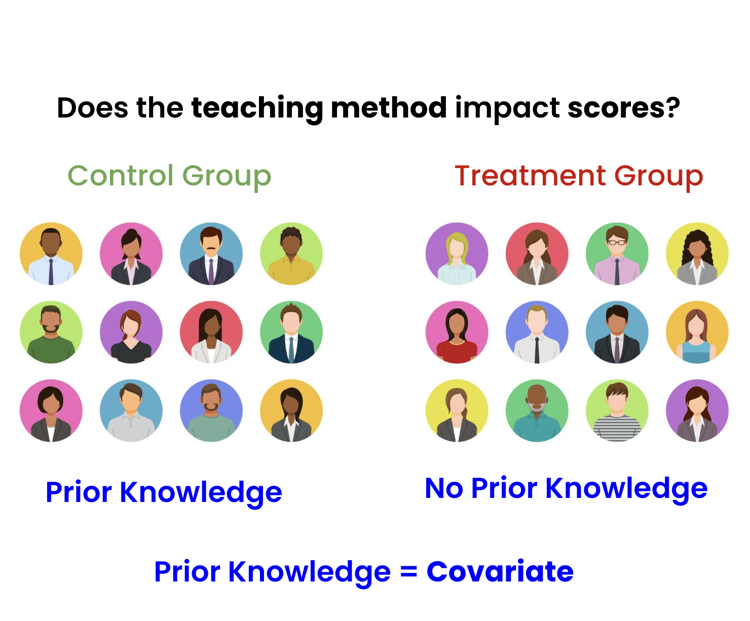
共變數：可能影響實驗結果，但不是主要關注
降低混雜的重要性
影響結果的精確度與效度

範例：教學法對測驗分數的影響

用測驗判定不同教學法是否影響成績。兩組在先備知識的分佈不均，因此此共變數造成混雜。

實驗資料範例

exp_plant_data = plant_growth_data[['Plant_ID', 'Fertilizer_Type', 'Growth_cm']]

   Plant_ID  Light_Condition  Fertilizer_Type  Growth_cm
0         1    Full Sunlight        Synthetic  16.489735
1         2    Partial Shade          Organic  18.361689
2         3    Full Sunlight        Synthetic  18.039459
3         4    Full Sunlight          Organic  12.682425
4         5    Full Sunlight          Organic  21.480601

共變數資料範例

covariate_data

   Plant_ID  Watering_Days_Per_Week
0         1                       6
1         2                       6
2         3                       4
3         4                       3
4         5                       7

結合實驗資料與共變數

merged_plant_data = pd.merge(exp_plant_data, covariate_data, on='Plant_ID')

   Plant_ID  Fertilizer_Type  Growth_cm  Watering_Days_Per_Week
0         1        Synthetic  16.489735                       6
1         2          Organic  18.361689                       6
2         3        Synthetic  18.039459                       4
3         4          Organic  12.682425                       3
4         5          Organic  21.480601                       7

對共變數進行調整

from statsmodels.formula.api import ols

model = ols('Growth_cm ~ Fertilizer_Type + Watering_Days_Per_Week',
            data=merged_plant_data).fit()

model.summary()

                            OLS Regression Results                            
==============================================================================
Dep. Variable:              Growth_cm   R-squared:                       0.011
Model:                            OLS   Adj. R-squared:                 -0.006
Method:                 Least Squares   F-statistic:                    0.6370
No. Observations:                 120   Prob (F-statistic):              0.531 <---
Df Residuals:                     117   Log-Likelihood:                -360.45
Df Model:                           2   AIC:                             726.9
Covariance Type:            nonrobust   BIC:                             735.3     
==============================================================================

進一步探索 ANCOVA 結果

                                       coef       std err             t       P>|t|      [0.025      0.975]
<hr />-----------------------------------------------------------------------------------------------------
Intercept                           19.3373         1.150        16.820       0.000      17.060      21.614
Fertilizer_Type[T.Synthetic]        -0.2796         0.913        -0.306       0.760 <--  -2.088       1.528
Watering_Days_Per_Week               0.2507         0.229         1.097       0.275 <--  -0.202       0.703
===========================================================================================================
Omnibus:                          14.446    Durbin-Watson:                   1.992
Prob(Omnibus):                     0.001    Jarque-Bera (JB):               18.267
Skew:                              0.675    Prob(JB):                     0.000108
Kurtosis:                          4.352    Cond. No.                         13.3
==================================================================================

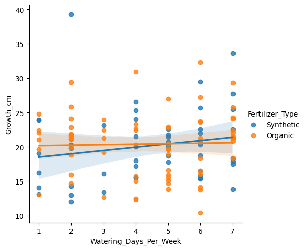
以共變數調整視覺化處理效果

import seaborn as sns
import matplotlib.pyplot as plt
sns.lmplot(x='Watering_Days_Per_Week', 
           y='Growth_cm', 
           hue='Fertilizer_Type', 
           data=merged_plant_data)
plt.show()

植物 lmplot

一起來練習吧！

Python 的實驗設計