比較時間序列的成長率

Manipulating Time Series Data in Python

Stefan Jansen

Founder & Lead Data Scientist at Applied Artificial Intelligence

比較股票表現

  • 股票價格序列:不同價位難以比較

  • 簡單作法:把價格序列正規化到起點為 100

  • 以序列第 1 筆相除後乘以 100

    • 相同起點

    • 價格皆相對於起點

    • 與起點的差異(百分點)

Manipulating Time Series Data in Python

單一序列正規化(1)

google = pd.read_csv('google.csv', parse_dates=['date'], index_col='date')

google.head(3)
             price
date
2010-01-04  313.06
2010-01-05  311.68
2010-01-06  303.83
first_price = google.price.iloc[0]  # int-based selection

first_price
313.06
first_price == google.loc['2010-01-04', 'price']
True
Manipulating Time Series Data in Python

單一序列正規化(2)

normalized = google.price.div(first_price).mul(100)

normalized.plot(title='Google Normalized Series')
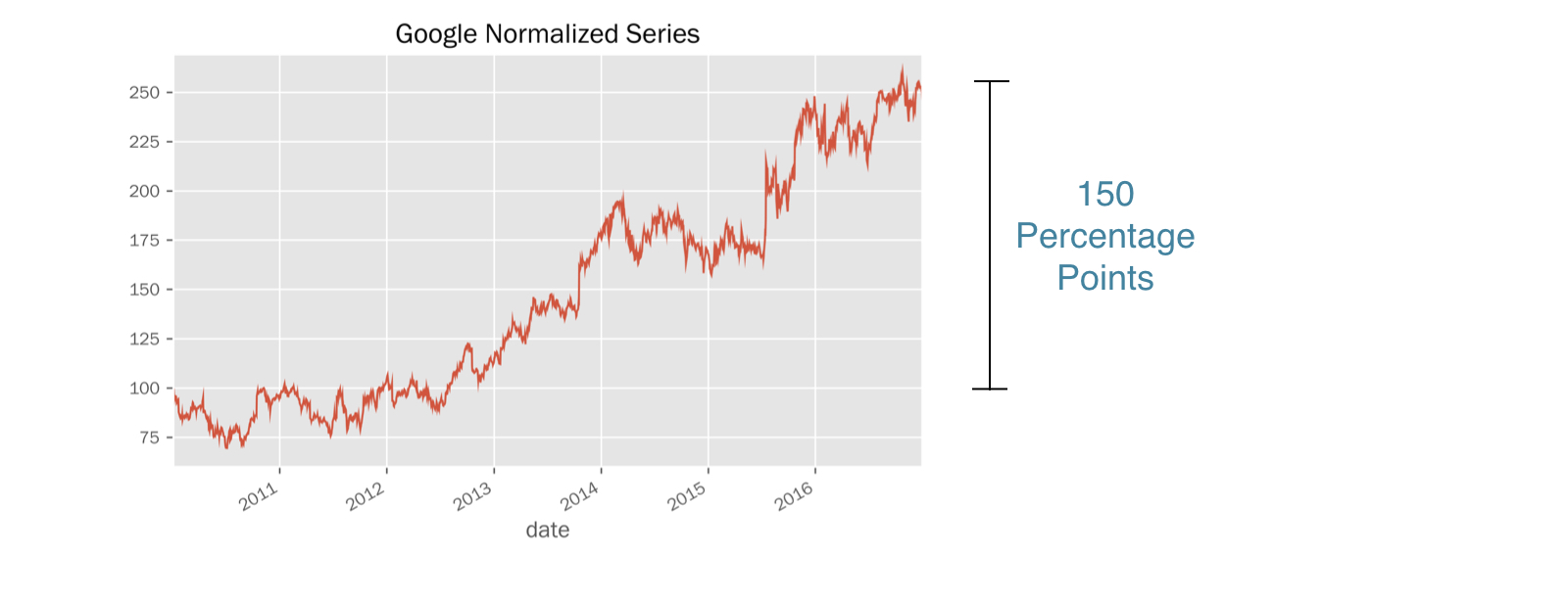
第 2 章:比較時間序列趨勢.017.png

Manipulating Time Series Data in Python

多序列正規化(1)

prices = pd.read_csv('stock_prices.csv',
                     parse_dates=['date'],
                     index_col='date')

prices.info()
DatetimeIndex: 1761 entries, 2010-01-04 to 2016-12-30
Data columns (total 3 columns):
AAPL    1761 non-null float64
GOOG    1761 non-null float64
YHOO    1761 non-null float64
dtypes: float64(3)
prices.head(2)
             AAPL    GOOG   YHOO
Date
2010-01-04  30.57  313.06  17.10
2010-01-05  30.63  311.68  17.23
Manipulating Time Series Data in Python

多序列正規化(2)

prices.iloc[0]
AAPL     30.57
GOOG    313.06
YHOO     17.10
Name: 2010-01-04 00:00:00, dtype: float64
normalized = prices.div(prices.iloc[0])

normalized.head(3)
                AAPL      GOOG      YHOO
Date
2010-01-04  1.000000  1.000000  1.000000
2010-01-05  1.001963  0.995592  1.007602
2010-01-06  0.985934  0.970517  1.004094
  • .div():自動對齊 Series 索引與 DataFrame 欄
Manipulating Time Series Data in Python

與基準比較(1)

index = pd.read_csv('benchmark.csv', parse_dates=['date'], index_col='date')

index.info()
DatetimeIndex: 1826 entries, 2010-01-01 to 2016-12-30
Data columns (total 1 columns):
SP500    1762 non-null float64
dtypes: float64(1)
prices = pd.concat([prices, index], axis=1).dropna()

prices.info()
DatetimeIndex: 1761 entries, 2010-01-04 to 2016-12-30
Data columns (total 4 columns):
AAPL     1761 non-null float64
GOOG     1761 non-null float64
YHOO     1761 non-null float64
SP500    1761 non-null float64
dtypes: float64(4)
Manipulating Time Series Data in Python

與基準比較(2)

prices.head(1)
             AAPL    GOOG   YHOO    SP500
2010-01-04  30.57  313.06  17.10  1132.99
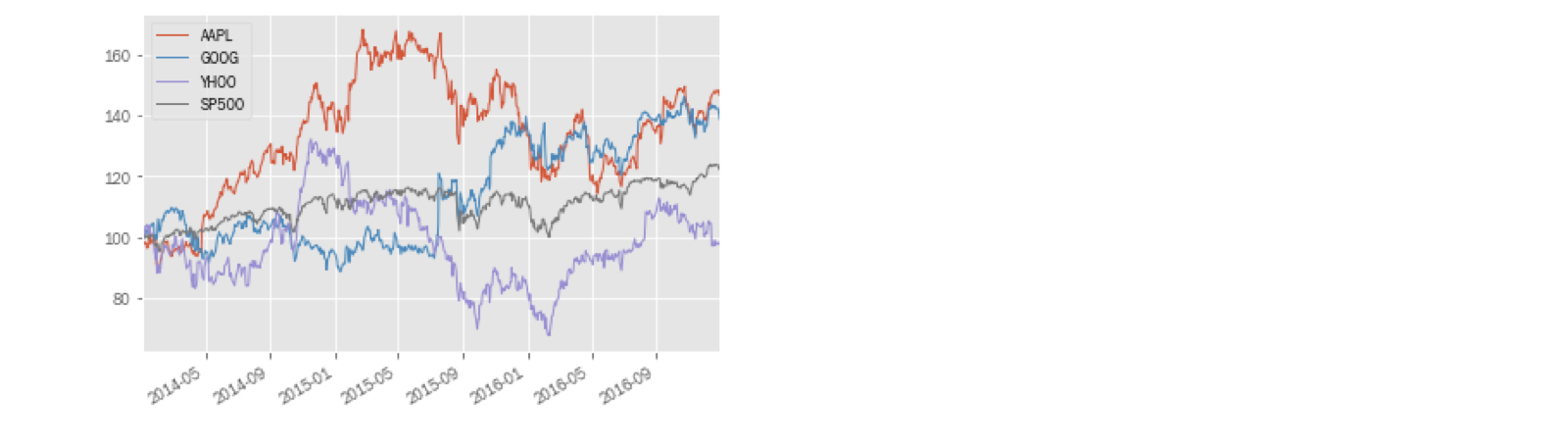
normalized = prices.div(prices.iloc[0]).mul(100)

normalized.plot()

第 2 章:比較時間序列趨勢.031.png

Manipulating Time Series Data in Python

繪製績效差異

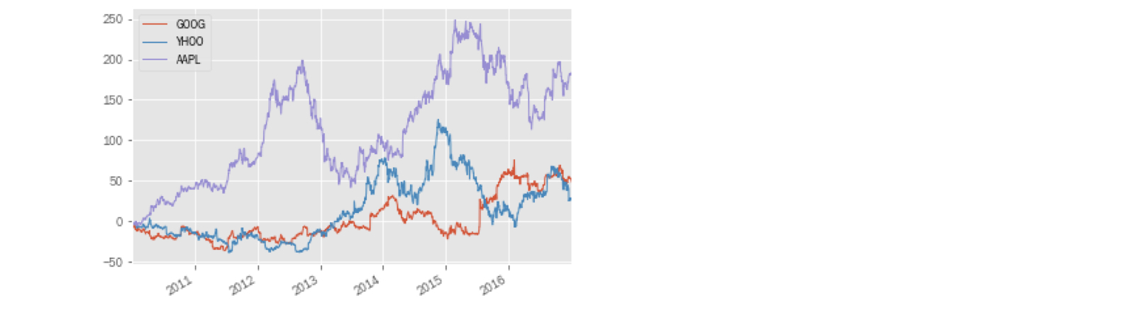
diff = normalized[tickers].sub(normalized['SP500'], axis=0)
                GOOG      YHOO      AAPL
2010-01-04  0.000000  0.000000  0.000000
2010-01-05 -0.752375  0.448669 -0.115294
2010-01-06 -3.314604  0.043069 -1.772895
  • .sub(..., axis=0):依索引對齊,將 Series 從各 DataFrame 欄相減
Manipulating Time Series Data in Python

繪製績效差異

diff.plot()

第 2 章:比較時間序列趨勢.035.png

Manipulating Time Series Data in Python

一起來練習吧!

Manipulating Time Series Data in Python

Preparing Video For Download...