延續 infer 流程

R 中的假設檢定

Richie Cotton

Data Evangelist at DataCamp

回顧：假設與資料集

$H_{0}$：30 歲以下的嗜好者比例與至少 30 歲的嗜好者比例相同。

$H_{A}$：30 歲以下的嗜好者比例與至少 30 歲的嗜好者比例不同。

alpha <- 0.1

stack_overflow_imbalanced %>% 
  count(hobbyist, age_cat, .drop = FALSE)

  hobbyist     age_cat    n
1       No At least 30    0
2       No    Under 30  191
3      Yes At least 30   15
4      Yes    Under 30 1025

回顧：工作流程

null_distn <- dataset %>% 
  specify() %>% 
  hypothesize() %>% 
  generate() %>% 
  calculate()

observed_stat <- dataset %>% 
  specify() %>% 
  calculate()

get_p_value(null_distn, observed_stat)

stack_overflow_imbalanced %>%
  specify(hobbyist ~ age_cat, success = "Yes") %>% 
  hypothesize(null = "independence")

Response: hobbyist (factor)
Explanatory: age_cat (factor)
Null Hypothesis: independence
# A tibble: 1,231 x 2
  hobbyist age_cat    
  <fct>    <fct>      
1 Yes      At least 30
2 Yes      At least 30
3 Yes      At least 30
4 Yes      Under 30   
5 Yes      At least 30
6 Yes      At least 30
7 No       Under 30   
# ... with 1,224 more rows

引入 generate()

$H_{0}$：30 歲以下的嗜好者比例與至少 30 歲的嗜好者比例相同。

若 $H_{0}$ 為真，則：

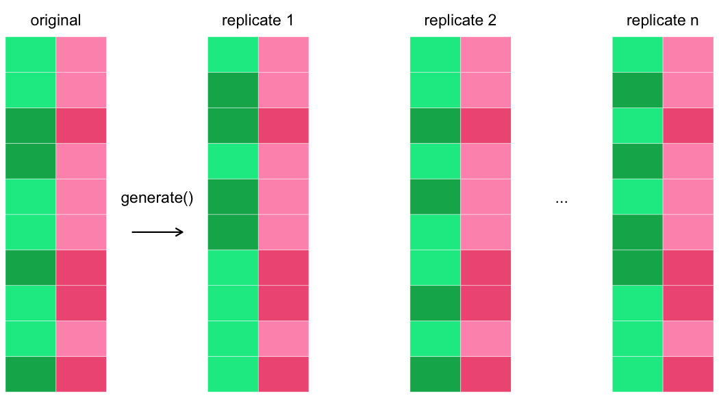
在每一列中，hobbyist 的值以相同機率出現在任一年齡類別。
要模擬此情況，可在固定年齡類別下，對 hobbyist 值做置換（洗牌）。

stack_overflow_imbalanced

# A tibble: 1,231 x 2
  hobbyist age_cat    
  <fct>    <fct>      
1 Yes      At least 30
2 Yes      At least 30
3 Yes      At least 30
4 Yes      Under 30   
5 Yes      At least 30
6 Yes      At least 30
7 No       Under 30   
# ... with 1,224 more rows

bind_cols(
  stack_overflow_imbalanced %>% 
    select(hobbyist) %>% 
    slice_sample(prop = 1),
  stack_overflow_imbalanced %>% 
    select(age_cat)
)

# A tibble: 1,231 x 2
  hobbyist age_cat    
  <fct>    <fct>      
1 Yes      At least 30
2 Yes      At least 30
3 No       At least 30
4 No       Under 30   
5 Yes      At least 30
6 Yes      At least 30
7 Yes      Under 30   
# ... with 1,224 more rows

產生多個重複樣本

左側為由指定欄位得到的兩欄網格。其右側顯示 generate，箭頭指向右邊三個兩欄網格，代表多個重複樣本。每個重複樣本的右欄與原始資料集相同，表示解釋變數不變；每個重複樣本的左欄不同，表示反應變數被置換。

generate()

generate() 會依虛無假設產生模擬資料。

對「independence」虛無假設，將 type 設為 "permute"。
對「point」虛無假設，將 type 設為 "bootstrap" 或 "simulate"。

stack_overflow_imbalanced %>%
  specify(hobbyist ~ age_cat, success = "Yes") %>% 
  hypothesize(null = "independence") %>% 
  generate(reps = 5000, type = "permute")

Response: hobbyist (factor)
Explanatory: age_cat (factor)
Null Hypothesis: independence
# A tibble: 6,155,000 x 3
# Groups:   replicate [5,000]
  hobbyist age_cat     replicate
  <fct>    <fct>           <int>
1 Yes      At least 30         1
2 Yes      At least 30         1
3 Yes      At least 30         1
4 Yes      Under 30            1
5 Yes      At least 30         1
6 Yes      At least 30         1
7 Yes      Under 30            1
# ... with 6,154,993 more rows

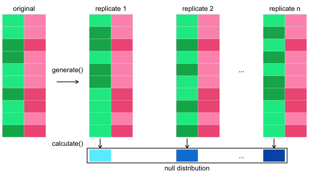
計算檢定統計量

上方為原始資料集與重複樣本的網格。下方標示 calculate，每個重複樣本下方有向下箭頭；箭頭下各有一個陰影格代表檢定統計量。所有重複樣本的統計量被框起並標示為「null distribution」。

calculate()

calculate() 會計算稱為「虛無分佈」的檢定統計量分佈。

null_distn <- stack_overflow_imbalanced %>%
  specify(
    hobbyist ~ age_cat, 
    success = "Yes"
  ) %>%
  hypothesize(null = "independence") %>%
  generate(reps = 5000, type = "permute") %>%
  calculate(
    stat = "diff in props", 
    order = c("At least 30", "Under 30")
  )

# A tibble: 5,000 x 2
  replicate    stat
      <int>   <dbl>
1         1  0.0896
2         2  0.0896
3         3 -0.180 
4         4  0.157 
5         5  0.0896
6         6 -0.113 
7         7  0.0221
# ... with 4,993 more rows

¹ `?calculate` 說明頁列出所有可用的檢定統計量。

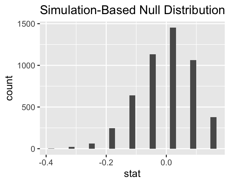
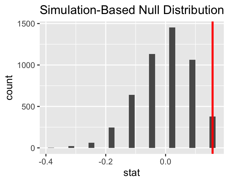
視覺化虛無分佈

visualize(null_distn)

虛無分佈的長條圖。左偏，且有 9 個不同的值。

null_distn %>% count(stat)

# A tibble: 9 x 2
     stat     n
    <dbl> <int>
1 -0.383      2
2 -0.315     22
3 -0.248     63
4 -0.180    246
5 -0.113    641
6 -0.0454  1132
7  0.0221  1453
8  0.0896  1063
9  0.157    378

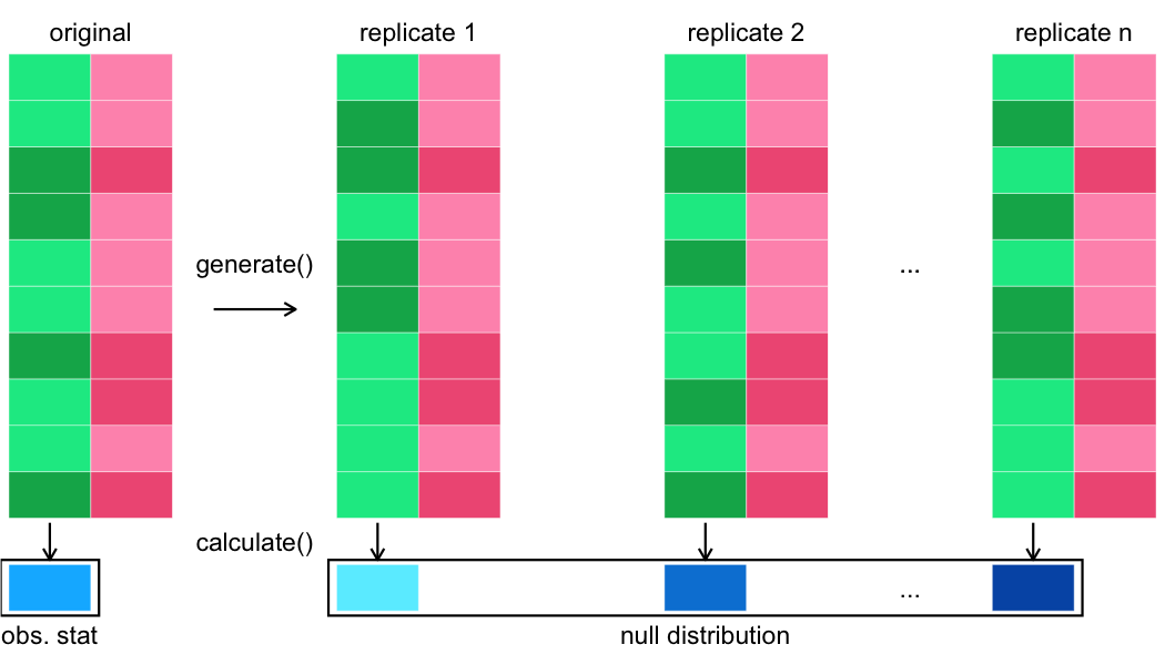
在原始資料集上計算統計量

與前一步相同的原始資料集與重複樣本網格，以及其下方的虛無分佈陰影格。本次在原始資料集下方也有向下箭頭，箭頭下方一個陰影格，並框選標示為「observed statistic」。

觀察統計量：specify() %>% calculate()

obs_stat <- stack_overflow_imbalanced %>%
  specify(hobbyist ~ age_cat, success = "Yes") %>%
  # hypothesize(null = "independence") %>%
  # generate(reps = 5000, type = "permute") %>%
  calculate(
    stat = "diff in props",
    order = c("At least 30", "Under 30")
  )

# A tibble: 1 x 1
   stat
  <dbl>
1 0.157

比較虛無分佈與觀察統計量

visualize(null_distn) +
  geom_vline(
    aes(xintercept = stat),
    data = observed_stat, 
    color = "red"
  )

虛無分佈的長條圖，另有一條紅色垂直線標示觀察統計量。此線位於長條圖最右側的長條上。

取得 p 值

get_p_value(
  null_distn, obs_stat, 
  direction = "two sided"   # 不是 alternative = "two.sided"
)

# A tibble: 1 x 1
  p_value
    <dbl>
1   0.151

# A tibble: 1 x 6
  statistic chisq_df p_value alternative lower_ci upper_ci
      <dbl>    <dbl>   <dbl> <chr>          <dbl>    <dbl>
1      2.79        1  0.0949 two.sided    0.00718   0.0217

一起來練習吧！

R 中的假設檢定