成對 t 檢定

R 中的假設檢定

Richie Cotton

Data Evangelist at DataCamp

美國共和黨總統資料集

state	county	repub_percent_08	repub_percent_12
Alabama	Bullock	25.69	23.51
Alabama	Chilton	78.49	79.78
Alabama	Clay	73.09	72.31
Alabama	Cullman	81.85	84.16
Alabama	Escambia	63.89	62.46
Alabama	Fayette	73.93	76.19
Alabama	Franklin	68.83	69.68
...	...	...	...

500 列；每列代表一次總統選舉的郡級得票。

¹ https://dataverse.harvard.edu/dataset.xhtml?persistentId=doi:10.7910/DVN/VOQCHQ

虛無與對立假設

問題：2008 年共和黨候選人的得票百分比是否低於 2012 年？

$H_{0}$: $\mu_{2008} - \mu_{2012} = 0$

$H_{A}$: $\mu_{2008} - \mu_{2012} < 0$

設定顯著水準 $\alpha = 0.05$。

這是成對資料，因為每個得票百分比都對應同一個郡。

由兩個樣本轉為一個樣本

sample_data <- repub_votes_potus_08_12 %>% 
  mutate(diff = repub_percent_08 - repub_percent_12)

ggplot(sample_data, aes(x = diff)) +
  geom_histogram(binwidth = 1)

diff 變數的直方圖——多數值介於 -10 到 10，並有些離群值。

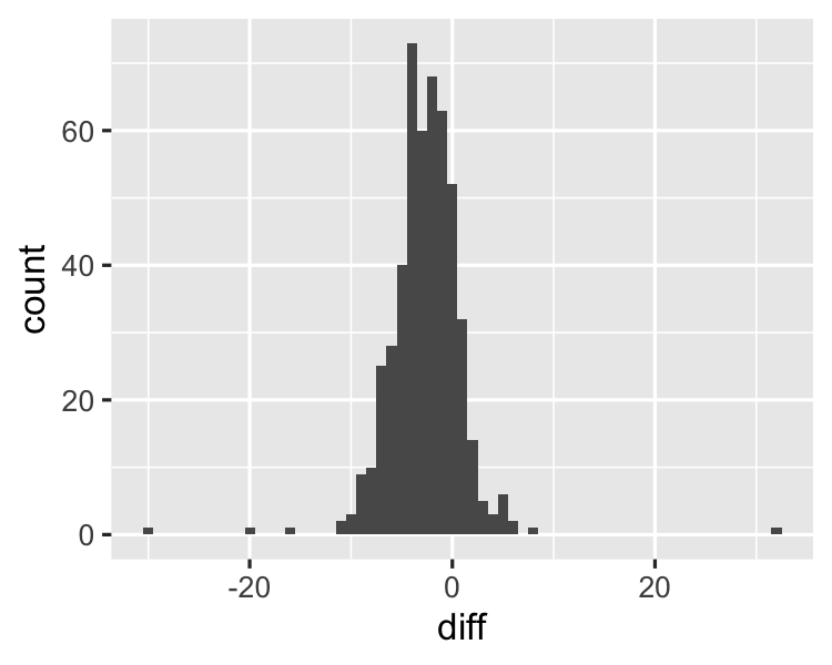
計算差值的樣本統計量

sample_data %>% 
  summarize(xbar_diff = mean(diff))

  xbar_diff
1 -2.643027

修正後的假設

舊版假設

$H_{0}$: $\mu_{2008} - \mu_{2012} = 0$

$H_{A}$: $\mu_{2008} - \mu_{2012} < 0$

新版假設

$H_{0}$: $\mu_{\text{diff}} = 0$

$H_{A}$: $ \mu_{\text{diff}} < 0$

$t = \dfrac{\bar{x}_{\text{diff}} - \mu_{\text{diff}}}{\sqrt{\dfrac{s_{diff}^2}{n_{\text{diff}}}}}$

$df = n_{diff} - 1$

計算 p 值

n_diff <- nrow(sample_data)

s_diff <- sample_data %>% 
  summarize(sd_diff = sd(diff)) %>%
  pull(sd_diff)

t_stat <- (xbar_diff - 0) / sqrt(s_diff ^ 2 / n_diff)

-16.06374

degrees_of_freedom <- n_diff - 1

$t = \dfrac{\bar{x}_{\text{diff}} - \mu_{\text{diff}}}{\sqrt{\dfrac{s_{\text{diff}}^2}{n_{\text{diff}}}}}$

$df = n_{\text{diff}} - 1$

p_value <- pt(t_stat, df = degrees_of_freedom)

2.084965e-47

用 t.test() 檢定兩個平均差

t.test(

  # Vector of differences
  sample_data$diff,

  # Choose between "two.sided", "less", "greater"
  alternative = "less",

  # Null hypothesis population parameter
  mu = 0

)

    One Sample t-test

data:  sample_data$diff
t = -16.064, df = 499, p-value < 2.2e-16
alternative hypothesis: true mean is less than 0
95 percent confidence interval:
     -Inf -2.37189
sample estimates:
mean of x 
-2.643027

t.test() 加上 paired = TRUE

t.test(
  sample_data$repub_percent_08,
  sample_data$repub_percent_12,
  alternative = "less",
  mu = 0,
  paired = TRUE
)

    Paired t-test

data:  sample_data$repub_percent_08 and 
       sample_data$repub_percent_12
t = -16.064, df = 499, p-value < 2.2e-16
alternative hypothesis: true difference in means 
                        is less than 0
95 percent confidence interval:
     -Inf -2.37189
sample estimates:
mean of the differences 
              -2.643027

未成對 t.test()

t.test(
  x = sample_data$repub_percent_08,
  y = sample_data$repub_percent_12,
  alternative = "less",
  mu = 0
)

未成對 t 檢定較容易發生偽陰性（統計力較低）。

    Welch Two Sample t-test

data:  sample_data$repub_percent_08 and 
       sample_data$repub_percent_12
t = -2.8788, df = 992.76, p-value = 0.002039
alternative hypothesis: true difference in means
                        is less than 0
95 percent confidence interval:
      -Inf -1.131469
sample estimates:
mean of x mean of y 
 56.52034  59.16337

一起來練習吧！

R 中的假設檢定