假設檢定與 z 分數

R 中的假設檢定

Richie Cotton

Data Evangelist at DataCamp

A/B 測試

  • Electronic Arts(EA)是一家電玩公司。
  • 2013 年他們發行 SimCity 5。
  • 目標是提高遊戲預購量。
  • 他們用 A/B 測試比較不同廣告情境。
  • 作法是把使用者分成「control」與「treatment」組。

Electronic Arts 大樓

1 圖片來源:「Electronic Arts」by majaX1 CC BY-NC-SA 2.0
R 中的假設檢定

零售網頁 A/B 測試

Control

SimCity 網站頁面,橫幅寫著「pre-order and get $20 off your next purchase」

Treatment

沒有橫幅的 SimCity 網站頁面

R 中的假設檢定

A/B 測試結果

  • treatment 組(無廣告)比 control 組(有廣告)多了 43.4% 的購買。
  • 「顯示廣告會提升銷售」的直覺其實不對。
  • 這個結果是「統計上顯著」還是巧合?
  • 你需要 EA 的資料來判定。
  • 可用 Sampling in R 的技巧加上本課內容來完成。
R 中的假設檢定

Stack Overflow Developer Survey 2020

library(dplyr)
glimpse(stack_overflow)
Rows: 2,261
Columns: 8
$ respondent         <dbl> 36, 47, 69, 125, 147, 152, 166, 170, 187, 196, 221,…
$ age_first_code_cut <chr> "adult", "child", "child", "adult", "adult", "adult…
$ converted_comp     <dbl> 77556, 74970, 594539, 2000000, 37816, 121980, 48644…
$ job_sat            <fct> Slightly satisfied, Very satisfied, Very satisfied,…
$ purple_link        <chr> "Hello, old friend", "Hello, old friend", "Hello, o…
$ age_cat            <chr> "At least 30", "At least 30", "Under 30", "At least…
$ age                <dbl> 34, 53, 25, 41, 28, 30, 28, 26, 43, 23, 24, 35, 37,…
$ hobbyist           <chr> "Yes", "Yes", "Yes", "Yes", "No", "Yes", "Yes", "Ye…
R 中的假設檢定

對母體平均的假設

一個假設:

資料科學家母體的年薪平均為 $110,000。

點估計(樣本統計量):

mean_comp_samp <- mean(stack_overflow$converted_comp)
mean_comp_samp <- stack_overflow %>% 
  summarize(mean_compensation = mean(converted_comp)) %>% 
  pull(mean_compensation)
119574.7
R 中的假設檢定

建立自助法分配

# Step 3. Repeat steps 1 & 2 many times
so_boot_distn <- replicate(
  n = 5000,
  expr = {
    # Step 1. Resample
    stack_overflow %>%
      slice_sample(prop = 1, replace = TRUE) %>%
      # Step 2. Calculate point estimate
      summarize(mean_compensation = mean(converted_comp)) %>% 
      pull(mean_compensation)
  }
)
1 自助法分配教於 Sampling in R 第 4 章
R 中的假設檢定

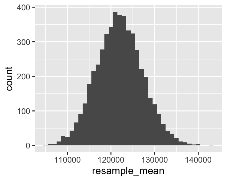
視覺化自助法分配

tibble(resample_mean = so_boot_distn) %>%
  ggplot(aes(resample_mean)) +
  geom_histogram(binwidth = 1000)

自助法分配的長條圖——呈鐘形,約介於 110000 與 140000 之間

R 中的假設檢定

標準誤

std_error <- sd(so_boot_distn)
5511.674
R 中的假設檢定

z 分數

$\text{standardized value} = \dfrac{\text{value} - \text{mean}}{\text{standard deviation}}$

$z = \dfrac{\text{sample stat} - \text{hypoth. param. value}}{\text{standard error}}$

$z = \dfrac{\$119,574.7 - \$110,000}{\$5511.67} = 1.737$

mean_comp_samp
119574.7
mean_comp_hyp <- 110000
std_error
5511.674
z_score <- (mean_comp_samp - mean_comp_hyp) / std_error
1.737171
R 中的假設檢定

檢驗假設

  • 1.737171 是高還是低?
  • 這就是本課的目標!
假設檢定的用途:

判斷樣本統計量是否接近或遠離預期(或「假設」)值。

R 中的假設檢定

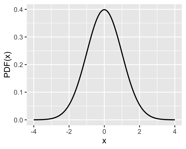
標準常態(z)分配

「標準常態分配」:平均為 0、標準差為 1 的常態分配。

tibble(x = seq(-4, 4, 0.01)) %>% 
  ggplot(aes(x)) +
  stat_function(fun = dnorm) +
  ylab("PDF(x)")

標準常態分配的 PDF 密度圖

R 中的假設檢定

一起來練習吧!

R 中的假設檢定

Preparing Video For Download...