假設的建立與分佈

Python 的 A/B 測試

Moe Lotfy, PhD

Principal Data Science Manager

定義假設

  • 假設是:

    • 對事件的解釋陳述
    • 進一步研究的起點
    • 你想要驗證的想法
  • 強而有力的假設:

    • 可檢驗、具宣告性、精簡且合乎邏輯
    • 能促進系統化迭代
    • 較易推廣並確認理解
    • 產出可行且聚焦的建議
Python 的 A/B 測試

假設格式

  • 一般 framing 格式:

    • 基於 X,我們相信若執行 Y
    • 則會發生 Z
    • 以指標 M 衡量
  • 對立假設範例:

    • 基於使用者經驗研究,我們相信若更新結帳頁面的設計
    • 則購買客戶的比例會上升
    • 以購買率衡量
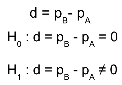
  • 虛無假設: …購買客戶的比例不會改變…
Python 的 A/B 測試

計算樣本統計量

# Calculate the number of users in groups A and B
n_A = checkout[checkout['checkout_page'] == 'A']['purchased'].count()
n_B = checkout[checkout['checkout_page'] == 'B']['purchased'].count()
print('Group A users:',n_A)
print('Group B users:',n_B)
Group A users: 3000
Group B users: 3000
# Calculate the mean purchase rates of groups A and B
p_A = checkout[checkout['checkout_page'] == 'A']['purchased'].mean()
p_B = checkout[checkout['checkout_page'] == 'B']['purchased'].mean()
print('Group A mean purchase rate:',p_A)
print('Group B mean purchase rate:',p_B)
Group A mean purchase rate: 0.820
Group B mean purchase rate: 0.847
Python 的 A/B 測試

模擬與繪製分佈

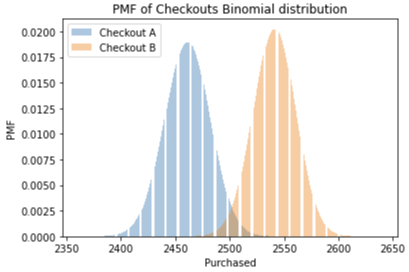
在購買機率為 p、試驗次數為 n 的情況下,購買人數服從二項分佈。

# Import binom from scipy library 
from scipy.stats import binom 
# Create x-axis range and Binomial distributions A and B
x = np.arange(n_A*p_A - 100, n_B*p_B + 100) 
binom_a = binom.pmf(x, n_A, p_A)
binom_b = binom.pmf(x, n_B, p_B) 
# Plot Binomial distributions A and B
plt.bar(x, binom_a, alpha=0.4, label='Checkout A')
plt.bar(x, binom_b, alpha=0.4, label='Checkout B')
plt.xlabel('Purchased')
plt.ylabel('PMF')
plt.title('PMF of Checkouts Binomial distribution')
plt.show()

結帳 A 與 B 組的二項分佈

Python 的 A/B 測試

中心極限定理

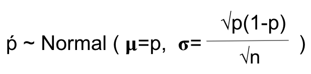
當樣本量足夠大時,樣本平均值 p 的分佈將

  • 以真實母體平均為中心,近似常態分佈
  • 標準差為平均數的標準誤
  • 不受原始資料分佈形狀影響

比例版中心極限定理公式

Python 的 A/B 測試

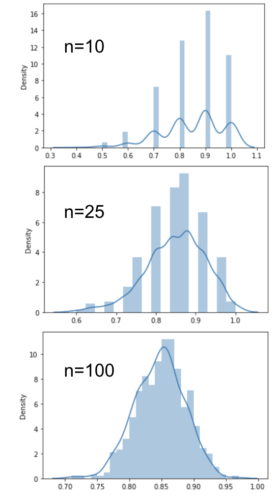
Python 的中心極限定理示範

# Set random seed for repeatability 
np.random.seed(47)
# Create an empty list to hold means
sampled_means = []
# Create loop to simulate 1000 sample means
for i in range(1000):
    # Take a sample of n=100
    sample = checkout['purchased'].sample(100,replace=True)
    # Get the sample mean and append to list
    sample_mean = np.mean(sample)
    sampled_means.append(sample_mean)
# Plot distribution
sns.displot(sampled_means, kde=True)
plt.show()

Python 展示中心極限定理。樣本量越大,分佈越趨近常態

Python 的 A/B 測試

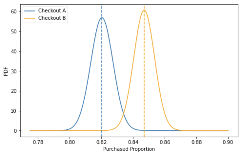
假設的數學表示

# Import norm from scipy library 
from scipy.stats import norm
# Create x-axis range and normal distributions A and B
x = np.linspace(0.775, 0.9, 500)
norm_a = norm.pdf(x, p_A, np.sqrt(p_A*(1-p_A) / n_A))
norm_b = norm.pdf(x, p_B, np.sqrt(p_B*(1-p_B) / n_B))
# Plot normal distributions A and B
sns.lineplot(x=x, y=norm_a, ax=ax, label='Checkout A')
sns.lineplot(x=x, y=norm_b, color='orange', \
             ax=ax, label= 'Checkout B')
ax.axvline(p_A, linestyle='--')
ax.axvline(p_B, linestyle='--')
plt.xlabel('Purchased Proportion')
plt.ylabel('PDF')
plt.legend(loc="upper left")
plt.show()

虛無與對立假設的平均差圖

虛無與對立假設的數學表述

Python 的 A/B 測試

一起來練習吧!

Python 的 A/B 測試

Preparing Video For Download...