具容量限制的設廠選址－案例研究 P4

Python 的供應鏈分析

Aaren Stubberfield

Supply Chain Analytics Mgr., Ingredion

模擬 vs. 敏感度分析

使用敏感度分析：

觀察需求與成本變動如何影響生產：
- 應該在哪裡增加生產？
- 生產會不會轉移到其他地區。
- 哪些地區的生產量較穩定？
比較同時多項變動與一次只變更一項的效果

模擬建模

我們可以把模擬測試套用到具容量限制的設廠選址模型。

可加入雜訊的輸入：

Demand
Variable costs
Fixed costs
Capacity

# Initialize Class
model = LpProblem(
            "Capacitated Plant Location Model",
             LpMinimize)

# Define Decision Variables
loc = ['A', 'B', 'C', 'D', 'E']
size = ['Low_Cap','High_Cap']
x = LpVariable.dicts(
       "production_", 
       [(i,j) for i in loc for j in loc],
       lowBound=0, upBound=None, cat='Continuous')
y = LpVariable.dicts(
      "plant_", [(i,s)for s in size for i in loc], 
       cat='Binary')

# Define Objective Function
model +=(lpSum([fix_cost.loc[i,s]*y[(i,s)]
               for s in size for i in loc])
       + lpSum([var_cost.loc[i,j]*x[(i,j)]
                for i in loc for j in loc]))

# Define the Constraints
for j in loc: model += 
  lpSum([x[(i, j)] for i in loc]) == demand.loc[
                                          j,'Dmd']
for i in loc: model += 
  lpSum([x[(i, j)] for j in loc]) <= lpSum(
                            [cap.loc[i,s]*y[(i,s)]
                             for s in size])
# Solve
model.solve()
print(LpStatus[model.status])

目標式：

model += (lpSum([fix_cost.loc[i,s]*y[(i,s)] for s in size for i in loc])
          + lpSum([(var_cost.loc[i,j] + normalvariate(0.5, 0.5))*x[(i,j)] 
                   for i in loc for j in loc]))

總需求：

for j in loc:
    rd = normalvariate(0, demand.loc[j,'Dmd']*.05)
    model += lpSum([x[(i,j)] for i in loc]) == (demand.loc[j,'Dmd']+rd)

程式碼範例－步驟 3

def run_pulp_model(fix_cost, var_cost, demand,
                   cap):
    # Initialize Class
    model = LpProblem(
              "Capacitated Plant Location Model", 
               LpMinimize)

    # Define Decision Variables
    loc = ['A', 'B', 'C', 'D', 'E']
    size = ['Low_Cap','High_Cap']
    x = LpVariable.dicts(
                "production_", 
                [(i,j) for i in loc for j in loc],
                lowBound=0, upBound=None,
                cat='Continuous')

    y = LpVariable.dicts(
               "plant_", 
               [(i,s) for s in size for i in loc], 
                cat='Binary')
    # Define the Constraints
    for j in loc: rd = normalvariate(
                       0, demand.loc[j,'Dmd']*.05)
        model += lpSum(
         [x[(i,j)] for i in loc]) == (
                           demand.loc[j,'Dmd']+rd)
    for i in loc: model += 
      lpSum([x[(i,j)] for j in loc]) \
        <= lpSum([cap.loc[i,s]*y[(i,s)] 
            for s in size])

    # Solve
    model.solve()
    o = {}
    for i in loc:
        o[i] = value(lpSum([x[(i, j)] for j in loc]))
    o['Obj'] = value(model.objective)
    return(o)

for i in range(100):
    output.append(run_pulp_model(fix_cost, var_cost, demand, cap))
df = pd.DataFrame(output)

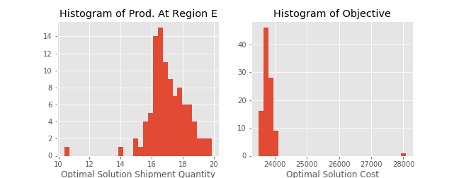
結果

import matplotlib.pyplot as plt
plt.title('Histogram of Prod. At Region E')
plt.hist(df['E'])
plt.show()

E 區生產與目標值的直方圖結果

重點回顧

具容量限制的設廠選址模型

模擬 vs. 敏感度分析
逐步走過程式碼範例

試試看！

Python 的供應鏈分析