使用 Python 的 statsmodels 進行迴歸分析:中級
Maarten Van den Broeck
Content Developer at DataCamp
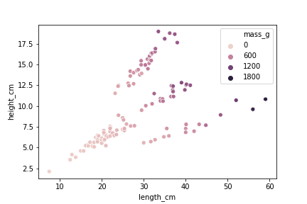
sns.scatterplot(x="length_cm",
                y="height_cm",
                data=fish,
                hue="mass_g")
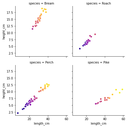
grid = sns.FacetGrid(data=fish,

                     col="species",

                     hue="mass_g",
                     col_wrap=2,

                     palette="plasma")
grid = sns.FacetGrid(data=fish,
col="species",
hue="mass_g", col_wrap=2,
palette="plasma")
grid.map(sns.scatterplot,
         "length_cm",
         "height_cm")
plt.show()
沒有交互作用
ols("mass_g ~ length_cm + height_cm + species + 0", data=fish).fit()
變數兩兩之間的二因交互作用
ols(
  "mass_g ~ length_cm + height_cm + species +
  length_cm:height_cm + length_cm:species + height_cm:species + 0", data=fish).fit()
三因交互作用(三者同時)
ols(
  "mass_g ~ length_cm + height_cm + species +
  length_cm:height_cm + length_cm:species + height_cm:species + length_cm:height_cm:species + 0", data=fish).fit()
等同於
ols(
  "mass_g ~ length_cm * height_cm * species + 0",
  data=fish).fit()
ols(
  "mass_g ~ (length_cm + height_cm + species) ** 2 + 0",
  data=fish).fit()
mdl_mass_vs_all = ols(
  "mass_g ~ length_cm * height_cm * species + 0",
  data=fish).fit()

length_cm = np.arange(5, 61, 5)
height_cm = np.arange(2, 21, 2)
species = fish["species"].unique()

p = product(length_cm, height_cm, species)

explanatory_data = pd.DataFrame(p,
                                columns=["length_cm",
                                         "height_cm",
                                         "species"])

prediction_data = explanatory_data.assign(
  mass_g = mdl_mass_vs_all.predict(explanatory_data))

print(prediction_data)
     length_cm  height_cm species       mass_g
0            5          2   Bream  -570.656437
1            5          2   Roach    31.449145
2            5          2   Perch    43.789984
3            5          2    Pike   271.270093
4            5          4   Bream  -451.127405
..         ...        ...     ...          ...
475         60         18    Pike  2690.346384
476         60         20   Bream  1531.618475
477         60         20   Roach  2621.797668
478         60         20   Perch  3041.931709
479         60         20    Pike  2926.352397

[480 rows x 4 columns]