含交互作用的預測

使用 Python 的 statsmodels 進行迴歸分析：中級

Maarten Van den Broeck

Content Developer at DataCamp

含交互作用的模型

mdl_mass_vs_both_inter = ols("mass_g ~ species + species:length_cm + 0",
                             data=fish).fit()

print(mdl_mass_vs_both_inter.params)

species[Bream]             -1035.3476
species[Perch]              -619.1751
species[Pike]              -1540.8243
species[Roach]              -329.3762
species[Bream]:length_cm      54.5500
species[Perch]:length_cm      38.9115
species[Pike]:length_cm       53.1949
species[Roach]:length_cm      23.3193

預測流程

from itertools import product

length_cm = np.arange(5, 61, 5)

species = fish["species"].unique()

p = product(length_cm, species)

explanatory_data = pd.DataFrame(p,
                                columns=["length_cm",
                                         "species"])

prediction_data = explanatory_data.assign(
 mass_g = mdl_mass_vs_both_inter.predict(explanatory_data))

print(prediction_data)

    length_cm species     mass_g
0           5   Bream  -762.5977
1           5   Roach  -212.7799
2           5   Perch  -424.6178
3           5    Pike -1274.8499
4          10   Bream  -489.8478
5          10   Roach   -96.1836
6          10   Perch  -230.0604
7          10    Pike -1008.8756
8          15   Bream  -217.0979
...
40         55   Bream  1964.9014
41         55   Roach   953.1833
42         55   Perch  1520.9556
43         55    Pike  1384.8933
44         60   Bream  2237.6513
45         60   Roach  1069.7796
46         60   Perch  1715.5129
47         60    Pike  1650.8677

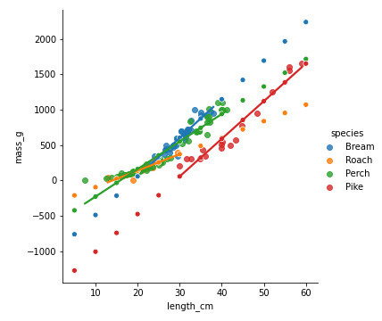
視覺化預測結果

sns.lmplot(x="length_cm",
           y="mass_g",
           data=fish,
           hue="species",
           ci=None)

sns.scatterplot(x="length_cm",
                y="mass_g",
                data=prediction_data,
                hue="species")

plt.show()

各物種分別顯示的魚長對質量散佈圖。

手動計算預測值

coeffs = mdl_mass_vs_both_inter.params

species[Bream]             -1035.3476
species[Perch]              -619.1751
species[Pike]              -1540.8243
species[Roach]              -329.3762
species[Bream]:length_cm      54.5500
species[Perch]:length_cm      38.9115
species[Pike]:length_cm       53.1949
species[Roach]:length_cm      23.3193

ic_bream, ic_perch, ic_pike, ic_roach,
slope_bream, slope_perch, slope_pike, slope_roach = coeffs

手動計算預測值

conditions = [
    explanatory_data["species"] == "Bream",
    explanatory_data["species"] == "Perch",
    explanatory_data["species"] == "Pike",
    explanatory_data["species"] == "Roach"    
]


ic_choices = [ic_bream, ic_perch, ic_pike, ic_roach]

intercept = np.select(conditions, ic_choices)


slope_choices = [slope_bream, slope_perch, slope_pike, slope_roach]

slope = np.select(conditions, slope_choices)

手動計算預測值

prediction_data = explanatory_data.assign(
 mass_g = intercept + slope * explanatory_data["length_cm"])

print(prediction_data)

    length_cm species     mass_g
0           5   Bream  -762.5977
1           5   Roach  -212.7799
2           5   Perch  -424.6178
3           5    Pike -1274.8499
4          10   Bream  -489.8478
5          10   Roach   -96.1836
...
43         55    Pike  1384.8933
44         60   Bream  2237.6513
45         60   Roach  1069.7796
46         60   Perch  1715.5129
47         60    Pike  1650.8677

prediction_data = explanatory_data.assign(
 mass_g = mdl_mass_vs_both_inter.predict(explanatory_data))

print(prediction_data)

    length_cm species     mass_g
0           5   Bream  -762.5977
1           5   Roach  -212.7799
2           5   Perch  -424.6178
3           5    Pike -1274.8499
4          10   Bream  -489.8478
5          10   Roach   -96.1836
...
43         55    Pike  1384.8933
44         60   Bream  2237.6513
45         60   Roach  1069.7796
46         60   Perch  1715.5129
47         60    Pike  1650.8677

一起來練習吧！

使用 Python 的 statsmodels 進行迴歸分析：中級