執行並追蹤插補

在 R 中處理遺漏值

Nicholas Tierney

Statistician

課程重點

用插補來理解資料結構

視覺化與探索插補值

透過插補來探索遺漏情形
追蹤遺漏值
將插補值與原始資料對照視覺化

用插補來理解資料結構

impute_below(c(5,6,7,NA,9,10))

5.00000  6.00000  7.00000  4.40271  9.00000 10.00000

impute_below

impute_below_if():

impute_below_if(data, is.numeric)

impute_below_at():

impute_below_at(data, vars(var1,var2))

impute_below_all():

impute_below_all(data)

追蹤遺漏值

df

# A tibble: 6 x 1
   var1
  <dbl>
1     5
2     6
3     7
4    NA
5     9
6    10

impute_below_all(df)

# A tibble: 6 x 1
   var1
  <dbl>
1  5   
2  6   
3  7   
4  4.40
5  9   
6 10

追蹤遺漏值

bind_shadow(df)

# A tibble: 6 x 2
   var1 var1_NA
  <dbl> <fct>  
1  5    !NA    
2  6    !NA    
3  7    !NA    
4  NA    NA     
5  9    !NA    
6 10    !NA

bind_shadow(df) %>% impute_below_all()

# A tibble: 6 x 2
   var1 var1_NA
  <dbl> <fct>  
1  5    !NA    
2  6    !NA    
3  7    !NA    
4  4.40 NA     
5  9    !NA    
6 10    !NA

用長條圖對照插補值與資料值

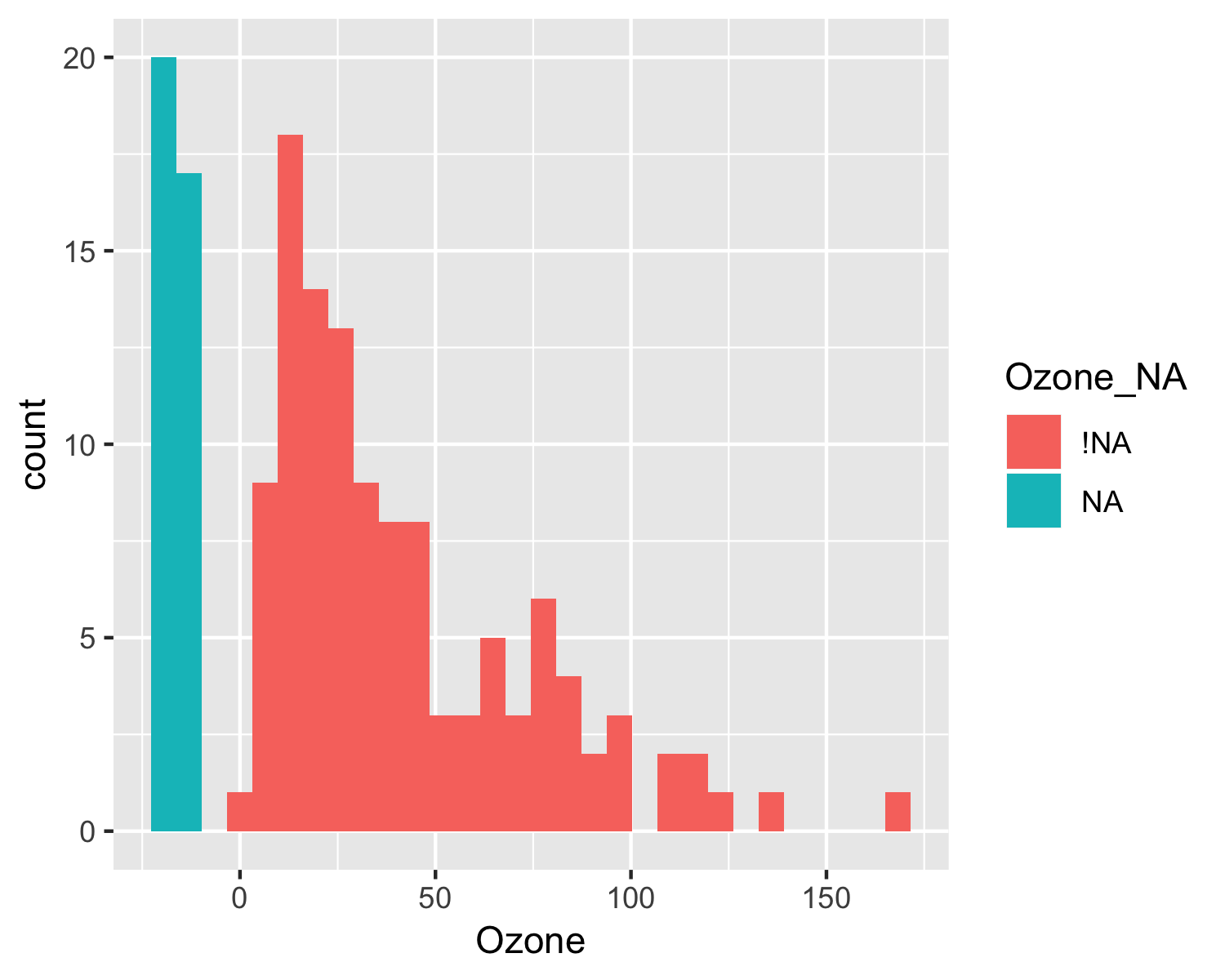
aq_imp <- airquality %>%
   bind_shadow() %>% 
   impute_below_all()

ggplot(aq_imp,
       aes(x = Ozone,
           fill = Ozone_NA)) + 
   geom_histogram()

用分面圖對照插補值與資料值

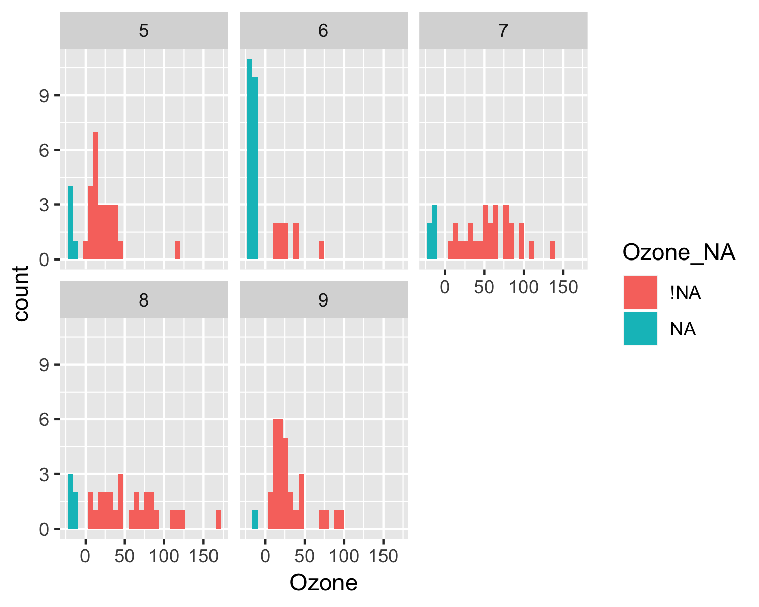
ggplot(aq_imp,
       aes(x = Ozone,
           fill = Ozone_NA)) + 
  geom_histogram() + 
  facet_wrap(~ Month)

用分面圖視覺化插補值

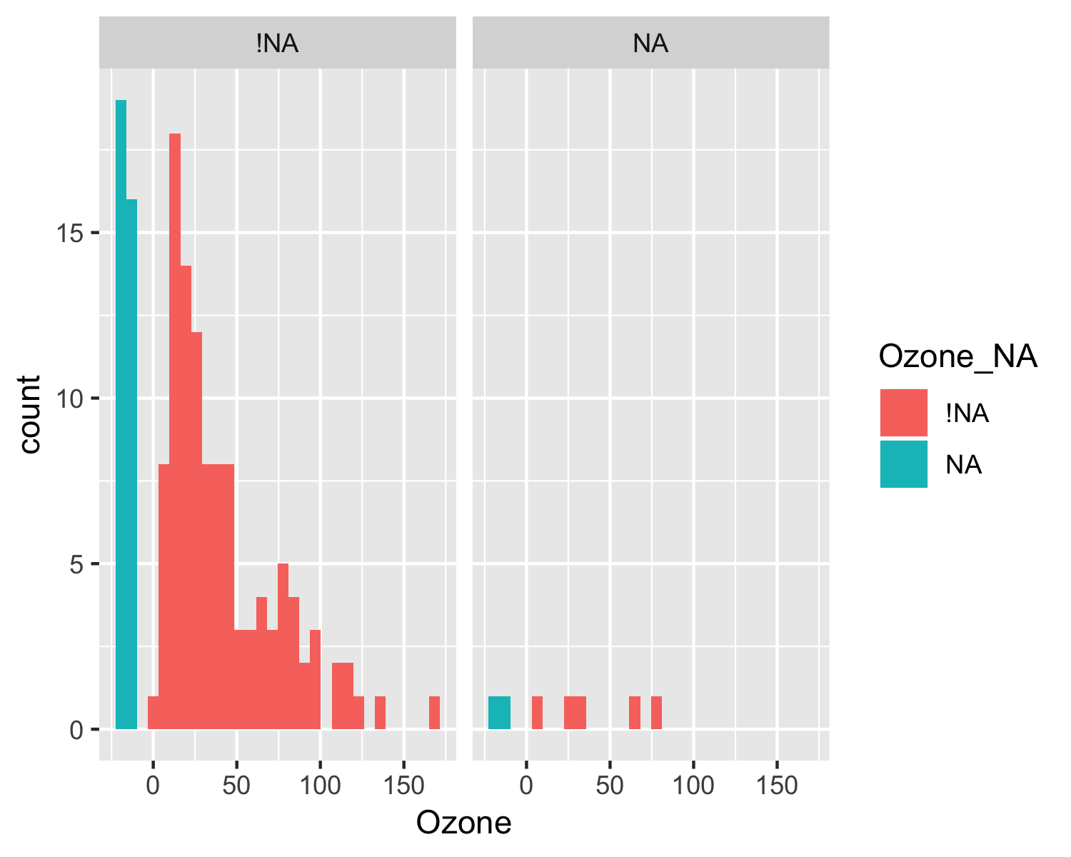
ggplot(aq_imp,
       aes(x = Ozone,
           fill = Ozone_NA)) + 
  geom_histogram() + 
  facet_wrap(~ Solar.R_NA)

用散佈圖對照插補值與資料值

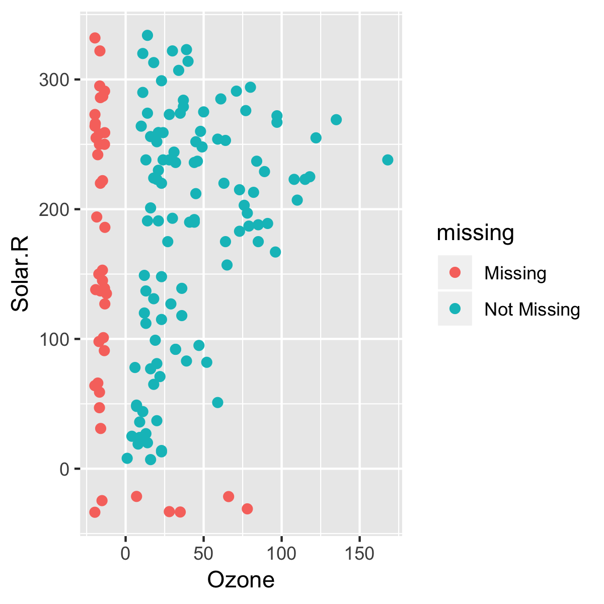
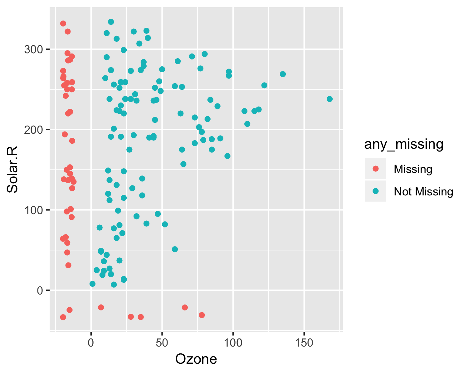
aq_imp <- airquality %>%
  bind_shadow() %>% 
  add_label_shadow() %>%
  impute_below_all()

ggplot(aq_imp,
       aes(x = Ozone,
           y = Solar.R,
           color = any_missing)) + 
  geom_point()

一起來練習吧！

在 R 中處理遺漏值