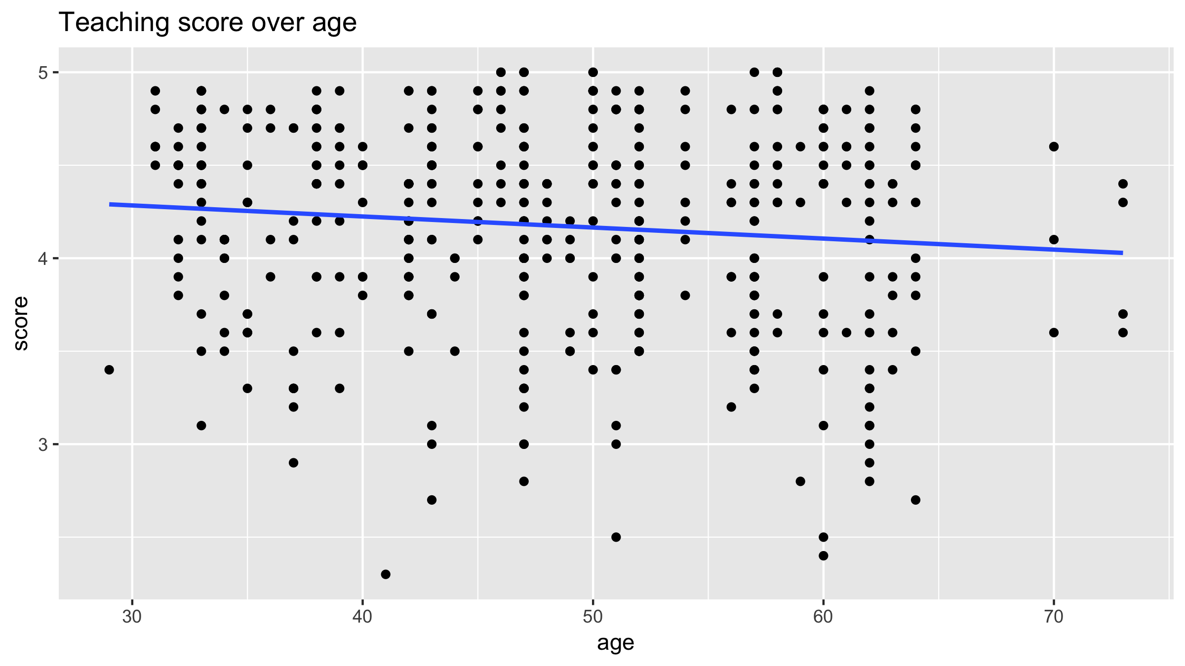
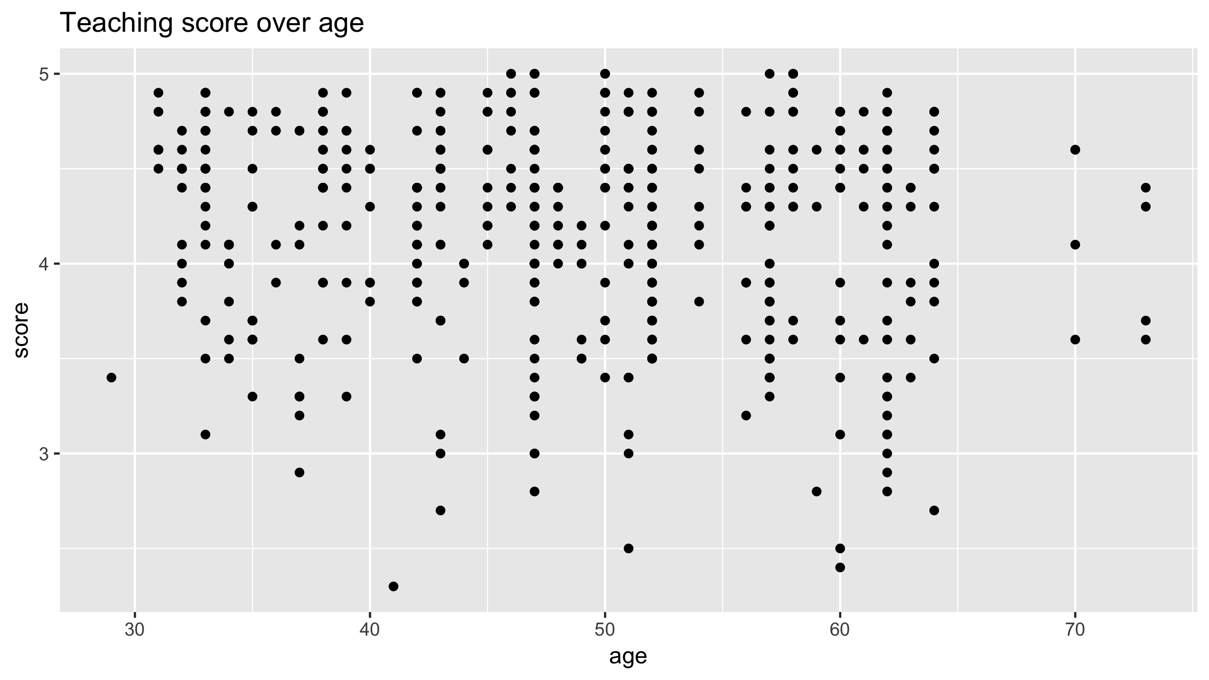
以年齡解釋教學評分

在 Tidyverse 中進行資料建模

Albert Y. Kim

Assistant Professor of Statistical and Data Sciences

複習：探索式資料視覺化

迴歸線

# Code to create scatterplot
ggplot(evals, aes(x = age, y = score)) +
  geom_point() + 
  labs(x = "age", y = "score", 
       title = "Teaching score over age")

# Add a "best-fitting" line
ggplot(evals, aes(x = age, y = score)) +
  geom_point() + 
  labs(x = "age", y = "score", 
       title = "Teaching score over age") +
  geom_smooth(method = "lm", se = FALSE)

迴歸線

複習：一般建模

真實：假設模型為 $y = f(\vec{x}) + \epsilon$
目標：給定 $y$ 與 $\vec{x}$，擬合模型 $\hat{f}(\vec{x})$ 來近似 $f(\vec{x})$，其中 $\hat{y} = \hat{f}(\vec{x})$ 為觀測值 $y$ 的擬合／預測值

基本線性迴歸建模

真實：
- 假設 $f(x) = \beta_0 + \beta_1 \cdot x$
- 觀測值 $y = f(x) + \epsilon = \beta_0 + \beta_1 \cdot x + \epsilon$
擬合：
- 假設 $\hat{f}(x) = \hat{\beta}_0 + \hat{\beta}_1 \cdot x$
- 擬合／預測值 $\hat{y} = \hat{f}(x) = \hat{\beta}_0 + \hat{\beta}_1 \cdot x$

回到迴歸線

藍色迴歸線的方程：$\hat{y} = \hat{f}(\vec{x}) = \hat{\beta}_0 + \hat{\beta}_1 \cdot x$

計算迴歸線的斜率與截距

使用公式形式 y ~ x：

# Fit regression model using formula of form: y ~ x
model_score_1 <- lm(score ~ age, data = evals)

# Output contents
model_score_1

Call:
lm(formula = score ~ age, data = evals)

Coefficients:
(Intercept)          age  
   4.461932    -0.005938

計算迴歸線的斜率與截距

使用公式形式 y ~ x，相當於 $\hat{y}= \hat{f}(\vec{x})$

# Fit regression model using formula of form: y ~ x
model_score_1 <- lm(score ~ age, data = evals)

# Output regression table using wrapper function:
get_regression_table(model_score_1)

# A tibble: 2 x 7
  term      estimate std_error statistic p_value...
  <chr>        <dbl>     <dbl>     <dbl>   <dbl>... 
1 intercept    4.46      0.127     35.2    0...
2 age         -0.006     0.003     -2.31   0.021...

一起來練習吧！

在 Tidyverse 中進行資料建模