核函式技巧

R 的支援向量機

Kailash Awati

Instructor

基本概念

設計轉換，讓問題可線性分離。
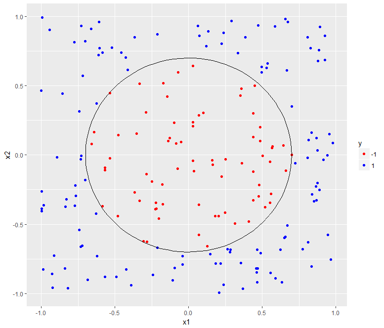
你會看到如何處理徑向可分的資料集。

第 3.3 章－徑向可分資料集與決策邊界

問題轉換

邊界方程為 $x_1 ^ 2 + x_2 ^ 2 = 0.49$
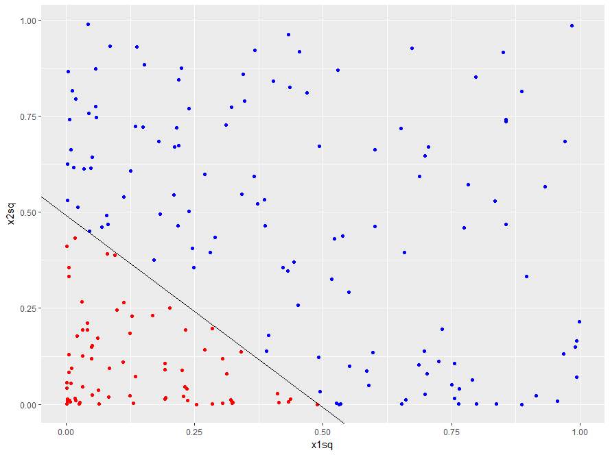
將 $x_1 ^ 2$ 映射到新變數 $X_1$，$x_2 ^ 2$ 映射到 $X_2$
在 $X_1 - X_2$ 空間中的邊界方程變為…
$X_1 + X_2 = 0.49$（一直線！）

在 X1-X2 空間繪圖－程式碼

使用 ggplot() 在 $X_1 - X_2$ 空間繪圖
邊界方程 $X_2 = -X_1 + 0.49$：
- $slope = -1$
- $yintercept = 0.49$

p <- ggplot(data = df4, aes(x = x1sq, y = x2sq, color = y)) + 
  geom_point() + 
  scale_color_manual(values = c("red", "blue")) +
  geom_abline(slope = -1, intercept = 0.49)

p

第 3.3 章－轉換後的徑向可分資料集與決策邊界

多項式核－第 1 部分

多項式核：(gamma * (u.v) + coef0) ^ degree
- degree 為多項式的次數
- gamma 與 coef0 為調參數
- u、v 為資料集中的向量（資料點）
我們可推測需要 2 次多項式（轉換）

核函式

SVM 的數學表述需要具備特定性質的轉換。
符合這些性質的函式稱為核函式。
核函式可視為向量內積的推廣。
核心想法：選用能把資料分得好的核。

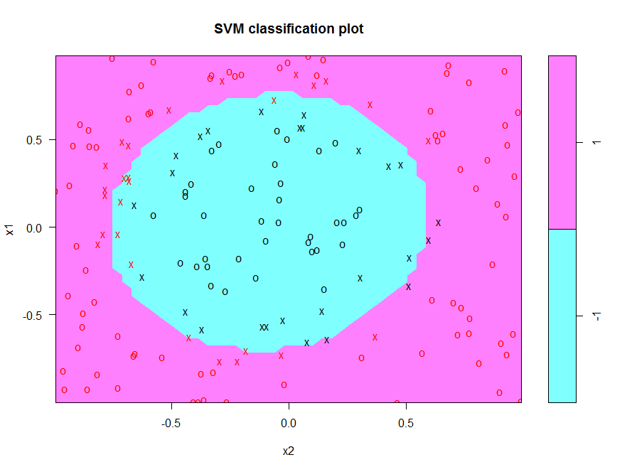
徑向可分資料集－二次核

80/20 訓練/測試切分
為徑向可分資料集建立二次 SVM：
- 設定 degree = 2
- cost、gamma、coef0 用預設值（1、1/2、0）

svm_model <- svm(y ~ ., data = trainset, type = "C-classification", kernel = "polynomial", degree = 2)
# Predictions
pred_test <- predict(svm_model, testset)
mean(pred_test == testset$y)

0.9354839

# Visualize model
plot(svm_model, trainset)

第 3.3 章－徑向可分資料集，預設 cost 的二次核，以 svm.plot 繪圖

一起來練習吧！

R 的支援向量機