視覺化線性 SVM

R 的支援向量機

Kailash Awati

Instructor

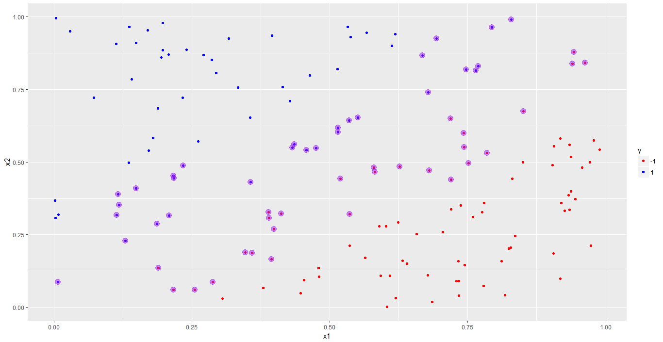
使用 ggplot() 繪製訓練資料。

# 視覺化訓練資料，使用顏色區分類別
p <- ggplot(data = trainset, aes(x = x1, y = x2, color = y)) +
     geom_point() +
     scale_color_manual(values = c("red", "blue"))
# 繪出圖形
p

使用 svm_model 的 index 標示支援向量。

# 取得支援向量
df_sv <- trainset[svm_model$index, ]
# 在圖上標示支援向量
p <- p + geom_point(data = df_sv,
                    aes(x = x1, y = x2),
                    color = "purple",
                    size = 4, alpha = 0.5)
# 顯示圖形
p

第 2.2 章－線性可分資料，預設 cost 線性 kernel 與支援向量

求邊界的斜率與截距：

由 svm_model 的 coefs 與 SV 建立權重向量 w。

# 建立權重向量
w <- t(svm_model$coefs) %*% svm_model$SV

斜率 = -w[1] / w[2]

# 計算斜率並存入變數
slope_1 <- -w[1] / w[2]

截距 = svm_model$rho / w[2]

# 計算截距並存入變數
intercept_1 <- svm_model$rho / w[2]

用前一張投影片計算的斜率與截距加入決策邊界。
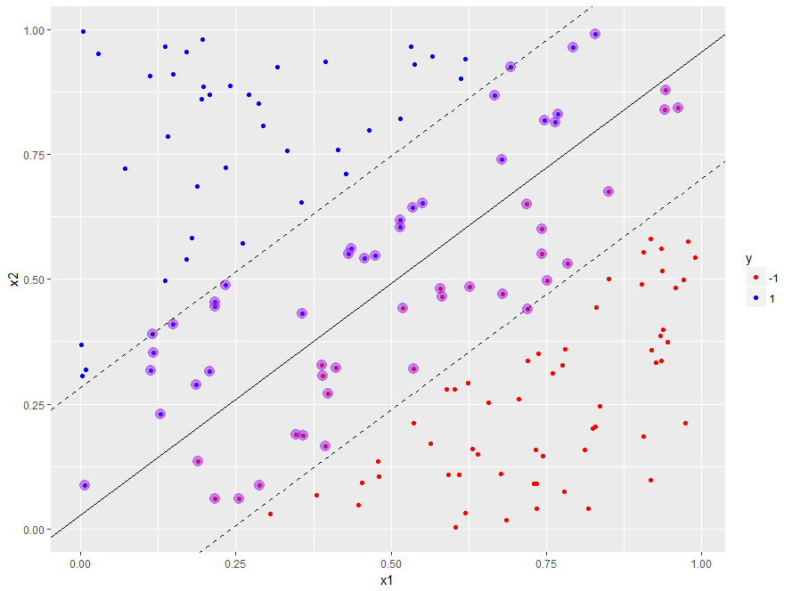
使用 geom_abline() 把決策邊界加到圖上。

# 依計算出的斜率與截距繪製決策邊界
p <- p + geom_abline(slope = slope_1,
                     intercept = intercept_1)

與決策邊界平行的邊際，在兩側各偏移 1 / w[2]。

# 在圖中加入邊際
p <- p + 
    geom_abline(slope = slope_1,
                intercept = intercept_1 - 1 / w[2],
                linetype = "dashed") + 
    geom_abline(slope = slope_1,
                intercept = intercept_1 + 1 / w[2],
                linetype = "dashed")
# 顯示圖形
p

第 2.2 章－線性可分資料，預設 cost 線性 kernel 含支援向量、決策與邊際邊界

Soft margin 分類器

容許邊界位置／形狀的不確定性
- 從不會完美線性
- 通常未知
我們的決策邊界是線性的，因此可縮小邊際

使用 svm plot() 視覺化決策邊界

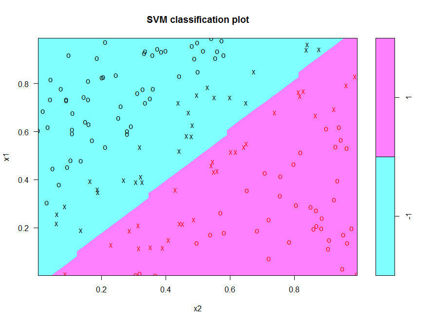
e1071 中的 svm plot() 提供簡便方式繪出決策邊界。

# 使用內建 plot 函式視覺化決策邊界
plot(x = svm_model,
     data = trainset)

第 2.2 章－線性可分資料，預設 cost 線性 kernel，使用 svm.plot 繪圖

一起來練習吧！

R 的支援向量機