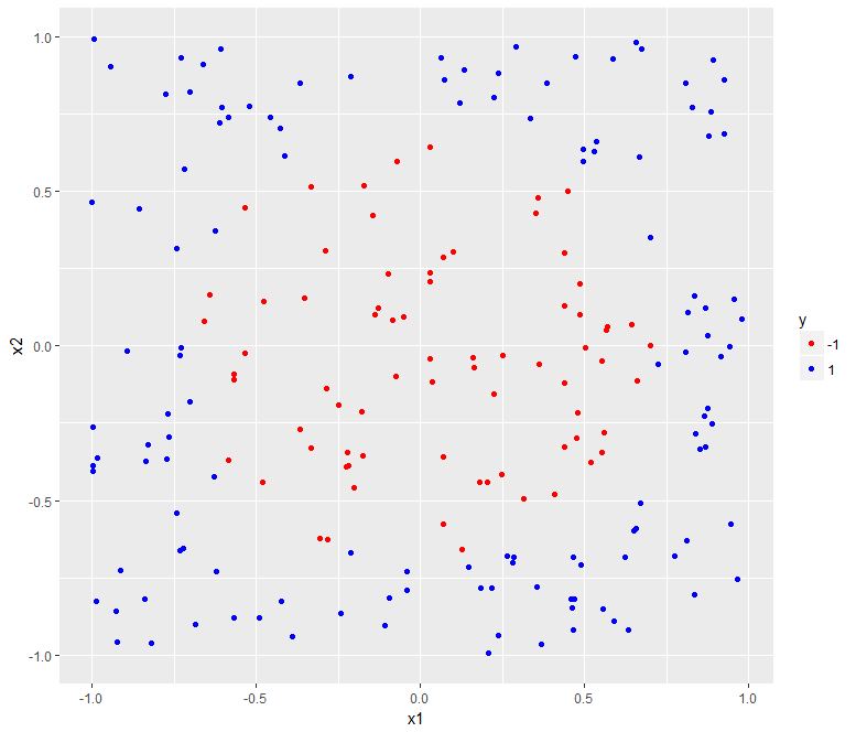
建立放射狀可分資料集

R 的支援向量機

Kailash Awati

Instructor

產生 2D 均勻分佈的點集

產生含 200 個點的資料集
- 2 個預測變數 x1、x2，在 -1 到 1 之間均勻分佈。

# Set required number of datapoints
n <- 200
# Set seed to ensure reproducibility
set.seed(42)

# Generate dataframe with 2 predictors x1 and x2 in (-1, 1)
df <- data.frame(x1 = runif(n, min = -1, max = 1),
                 x2 = runif(n, min = -1, max = 1))

建立圓形邊界

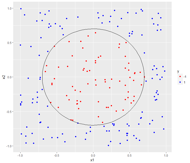
建立半徑 0.7 的圓形決策邊界。
類別變數 y 依點在邊界內外為 -1 或 +1。

radius <- 0.7
radius_squared <- radius ^ 2

#categorize data points depending on location wrt boundary
df$y <- factor(ifelse(df$x1 ^ 2 + df$x2 ^ 2 < radius_squared, -1, 1),
               levels = c(-1, 1))

繪製資料集

用 ggplot 視覺化。

library(ggplot2)

將預測變數畫在 2 軸上；用顏色區分類別。

# Build plot
p <- ggplot(data = df, aes(x = x1, y = x2, color = y)) + 
     geom_point() + 
     scale_color_manual(values = c("-1" = "red", "1" = "blue")) 
# Display plot 
p

第 3.1 章－放射狀可分資料集

加入圓形邊界－第 1 部分

我們要建立一個產生圓的函式

# Function generates dataframe with points
# lying on a circle of radius r
circle <- 
  function(x1_center, x2_center, r, npoint = 100) {

  # Angular spacing of 2*pi/npoint between points
  theta <- seq(0, 2 * pi, length.out = npoint)
  x1_circ <- x1_center + r * cos(theta)
  x2_circ <- x2_center + r * sin(theta)

  data.frame(x1c = x1_circ, x2c = x2_circ)
}

加入圓形邊界－第 2 部分

要把邊界加到圖上：
- 用 circle() 產生邊界。
- 用 geom_path() 把邊界加入圖中。

# Generate boundary
boundary <- circle(x1_center = 0,
                   x2_center = 0,
                   r = radius)
# Add boundary to previous plot
p <- p + 
     geom_path(data = boundary,
               aes(x = x1c, y = x2c),
               inherit.aes = FALSE)
# Display plot
p

第 3.1 章－含決策邊界的放射狀可分資料集

一起來練習吧！

R 的支援向量機