使用 flexmix 的單變量高斯混合模型

R 中的混合模型

Victor Medina

Researcher at The University of Edinburgh

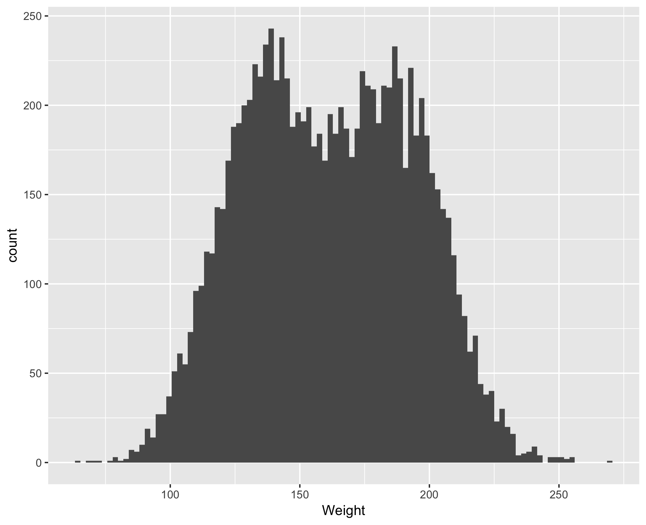
gender %>% 
  ggplot(aes(x = Weight)) + geom_histogram(bins = 100)

以混合模型建模

哪個機率分佈合適？
- 單變量高斯分佈
應該考慮多少子族群？
- 2 個叢集
參數與其估計為何？
- 以 flexmix 實作的 EM 演算法估計平均數、標準差與比例

flexmix 函式

flexmix(formula, data, k, model, control, ...)

formula：要擬合的模型描述（$variable \sim 1$）
data：資料框
k：叢集數
model：指定分佈（FLXMCnorm1、FLXMCmvnorm、FLXMCmvbinary、FLXMRglm、FLXMCmvpois）
control：指定最大反覆次數、收斂容許誤差等

fit_mixture <- flexmix(Weight ~ 1, # the means and sds are constant
                data = gender, # the data frame
                k = 2, # the number of clusters,
                model = FLXMCnorm1(), # univariate Gaussian    
                control = list(tol = 1e-15, # tolerance for EM stop
                               verbose = 1, # show partial results
                               iter = 1e4)) # max number of iterations

Classification: weighted 
   1 Log-likelihood :  -48880.0782 
   2 Log-likelihood :  -48880.0745 
   3 Log-likelihood :  -48880.0732 
   4 Log-likelihood :  -48880.0727
   .    .   .   .   .   .   .   .
3454 Log-likelihood :  -48518.3717 
3455 Log-likelihood :  -48518.3717 
3456 Log-likelihood :  -48518.3717 
3457 Log-likelihood :  -48518.3717 
converged

比例：prior 函式

proportions <- prior(fit_mixture)
proportions

0.4929668 0.5070332

兩個分佈一起看

parameters(fit_mixture)

                    Comp.1    Comp.2
coef.(Intercept) 135.54652 186.61583
sigma             18.94726  19.96097

分別查看

comp_1 <- parameters(fit_mixture, component = 1)
comp_2 <- parameters(fit_mixture, component = 2)
comp_2

                    Comp.2
coef.(Intercept) 186.61583
sigma             19.96097

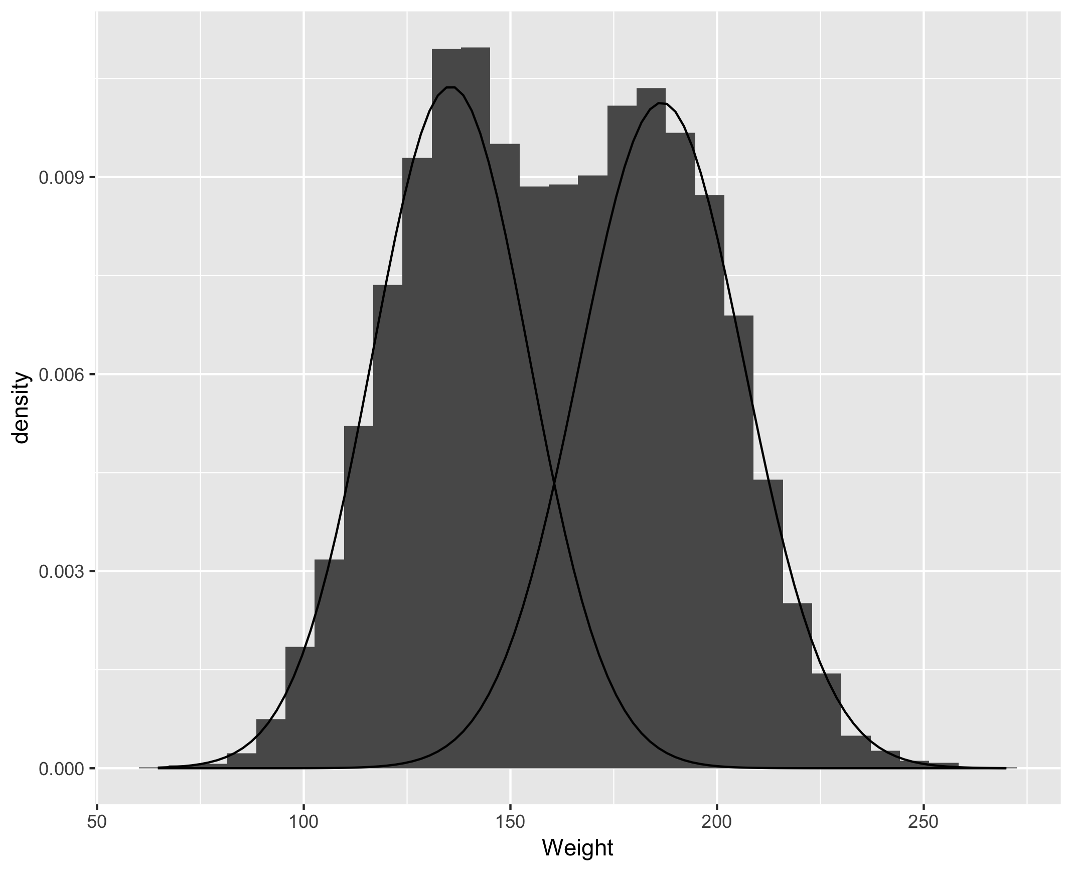
視覺化結果分佈

gender %>%
   ggplot() + geom_histogram(aes(x = Weight, y = ..density..)) + 
   stat_function(geom = "line", fun = fun_prop, 
                 args = list(mean = comp_1[1], 
                             sd = comp_1[2], 
                             proportion = proportions[1])) +
   stat_function(geom = "line", fun = fun_prop, 
                 args = list(mean = comp_2[1], 
                             sd = comp_2[2], 
                             proportion = proportions[2]))

posterior 函式

posterior(fit_mixture) %>% head()

             [,1]      [,2]
[1,] 6.836341e-06 0.9999932
[2,] 4.421760e-01 0.5578240
[3,] 5.994160e-04 0.9994006
[4,] 1.998798e-04 0.9998001
[5,] 1.547774e-03 0.9984522
[6,] 7.544450e-01 0.2455550

clusters 函式

clusters(fit_mixture) %>% head()

2 2 2 2 2 1

指派比較

table(gender$Gender, clusters(fit_mixture))

            1    2
  Female 4500  500
  Male    444 4556

一起來練習吧！

R 中的混合模型