Posterior estimation & inference
Bayesian Modeling with RJAGS

Alicia Johnson
Associate Professor, Macalester College
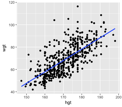
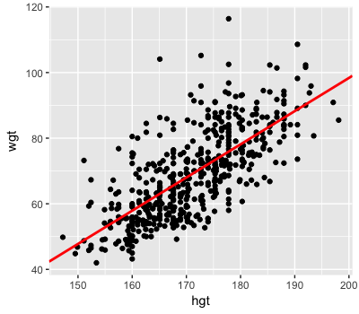
Bayesian regression model
Posterior point estimation
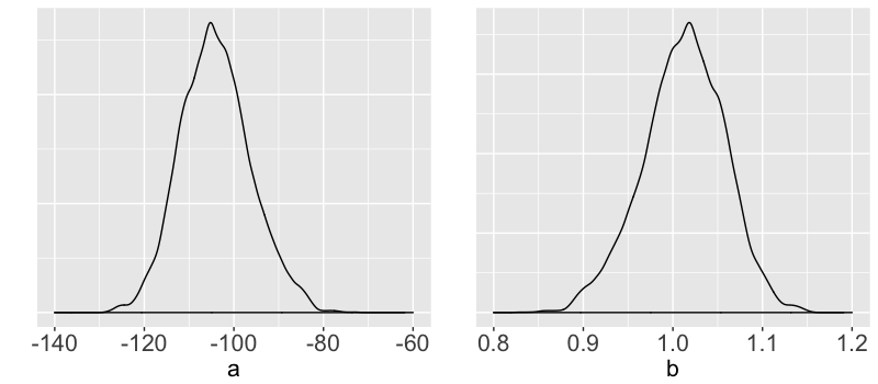
Posterior point estimation
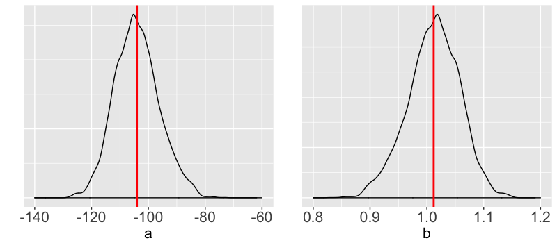
Posterior point estimation
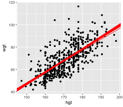
Posterior uncertainty
Posterior credible intervals
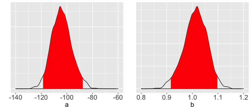
Posterior credible intervals
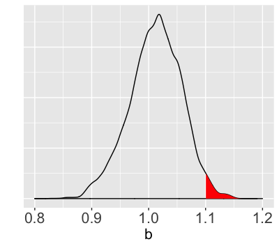
Posterior probabilities