Model the data

Differential Expression Analysis with limma in R

John Blischak

Instructor

Ready for analysis

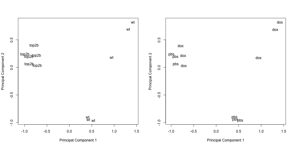
# Plot principal components labeled by genotype
plotMDS(eset, labels = pData(eset)[, "genotype"], gene.selection = "common")
# Plot principal components labeled by treatment
plotMDS(eset, labels = pData(eset)[, "treatment"], gene.selection = "common")

Steps for differential expression analysis

Build the design matrix with model.matrix
Contruct the contrasts matrix with makeContrasts
Test the contrasts with lmFit, contrasts.fit, and eBayes

Group-means model for doxorubicin study

$$ Y = \beta_1 X_1 + \beta_2 X_2 + \beta_3 X_3 + \beta_4 X_4 + \epsilon $$

$\beta_1$ - Mean expression level in top2b mice treated with dox
$\beta_2$ - Mean expression level in top2b treated with pbs
$\beta_3$ - Mean expression level in wt mice treated with dox
$\beta_4$ - Mean expression level in wt mice treated with pbs

Contrasts for doxorubicin study

	$\beta_1$	$\beta_2$	$\beta_3$	$\beta_4$
`genotype`	top2b	top2b	wt	wt
`treatment`	dox	pbs	dox	pbs

Response of wild type mice to dox treatment: $\beta_3 - \beta_4 = 0$
Response of Top2b null mice to dox treatment: $\beta_1 - \beta_2 = 0$
Differences between Top2b null and wild type mice in response to dox treatment: $(\beta_1 - \beta_2) - (\beta_3 - \beta_4) = 0$

Testing the doxorubicin study

Fit the model coefficients with lmFit
Fit the contrasts with contrasts.fit
Calculate the t-statistics with eBayes

# Summarize results
results <- decideTests(fit2)
summary(results)

# Create a Venn diagram
vennDiagram(results)

Let's practice!

Differential Expression Analysis with limma in R