Choosing the number of components
Multivariate Probability Distributions in R

Surajit Ray
Professor, University of Glasgow
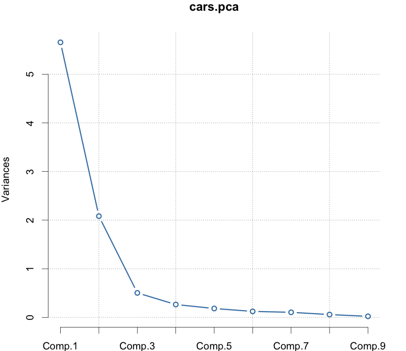
Using the scree plot
![]()
Calculating cumulative proportional variance
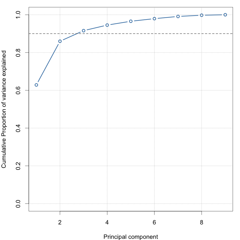
Calculating cumulative proportional variance
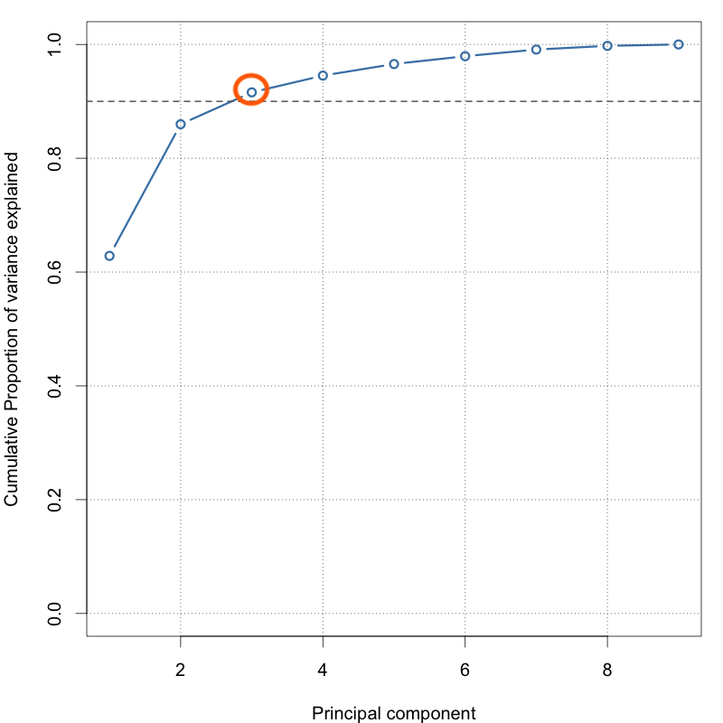
3 PCs explain 90 percent of the variation

