Multi-dimensional Scaling

Multivariate Probability Distributions in R

Surajit Ray

Professor, University of Glasgow

What is Multidimensional Scaling?

Classical multidimensional scaling (MDS) or principal coordinates analysis
- INPUT matrix of distances
- OUTPUT Set of points in given dimensions such that the distances closely match the INPUT distances
- cmdscale() function
```
cmdscale(d, k = 2, ...)
```
Non-metrics scaling
- isoMDS()
- sammon()

US City distance example

data("UScitiesD")
UScitiesD

               Atlanta Chicago Denver Houston LosAngeles Miami NewYork SanFrancisco Seattle
Chicago           587                                                                     
Denver           1212     920                                                             
Houston           701     940    879                                                      
LosAngeles       1936    1745    831    1374                                              
Miami             604    1188   1726     968       2339                                   
NewYork           748     713   1631    1420       2451  1092                             
SanFrancisco     2139    1858    949    1645        347  2594    2571                     
Seattle          2182    1737   1021    1891        959  2734    2408          678        
Washington.DC     543     597   1494    1220       2300   923     205         2442    2329

MDS on US city distance dataset

usloc <- cmdscale(UScitiesD)
usloc

               [,1]   [,2]
Atlanta        -719  143.0
Chicago        -382 -340.8
Denver          482  -25.3
Houston        -161  572.8
LosAngeles     1204  390.1
Miami         -1134  581.9
NewYork       -1072 -519.0
SanFrancisco   1421  112.6
Seattle        1342 -579.7
Washington.DC  -980 -335.5

ggplot(data = data.frame(usloc), aes(x = X1, y = X2, label = rownames(usloc))) + 
    geom_text()

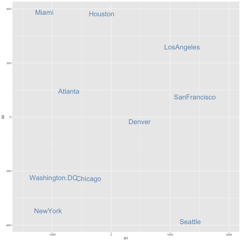
US cities MDS output

Plot of output from cmdscale

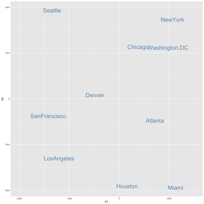
Plot after rotation

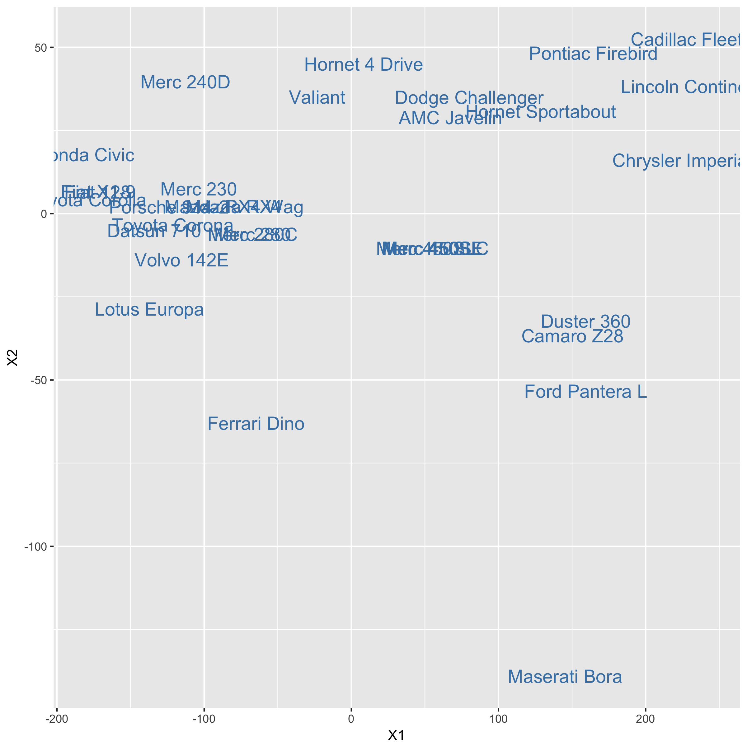
cars.dist <- dist(mtcars)

cars.mds <- cmdscale(cars.dist, k = 2)

cars.mds <- data.frame(cars.mds)
ggplot(data = cars.mds, aes(x = X1, y = X2, label = rownames(cars.mds))) + geom_text()

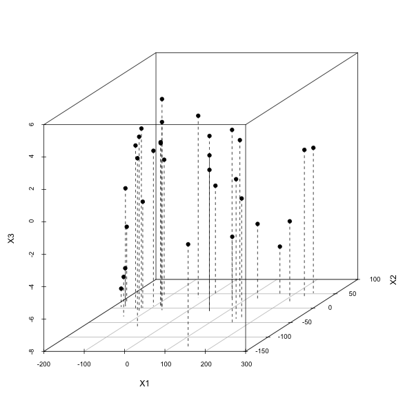
Multidimensional scaling in more than two dimensions

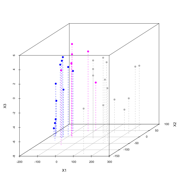
cars.dist <- dist(mtcars)

cmds3 <- data.frame(cmdscale(cars.dist, k = 3)) 

scatterplot3d(cmds3, type = "h", pch = 19, lty.hplot = 2)

Multidimensional scaling in more than two dimensions

cars.dist <- dist(mtcars)

cmds3 <- data.frame(cmdscale(cars.dist, k = 3)) 

scatterplot3d(cmds3, type = "h", pch = 19, lty.hplot = 2, color = mtcars$cyl)

Now let's try using MDS!

Multivariate Probability Distributions in R