Interpreting PCA outputs

Multivariate Probability Distributions in R

Surajit Ray

Reader, University of Glasgow

Attributes of princomp object

cars.pca <- princomp(mtcars.sub, cor = TRUE, scores = TRUE)

attributes(cars.pca)

$names
[1] "sdev" "loadings" "center" "scale" "n.obs" "scores" "call"

Interpretation of loadings

All 8 components

 cars.pca$loadings # or loadings(cars.pca)

Loadings:
     Comp.1 Comp.2 Comp.3 Comp.4 Comp.5 Comp.6 Comp.7 Comp.8 Comp.9
mpg   0.393        -0.221        -0.321  0.720  0.381  0.125 -0.115
cyl  -0.403        -0.252         0.117  0.224  0.159 -0.810 -0.163
disp -0.397                0.339 -0.487         0.182         0.662
hp   -0.367 -0.269               -0.295  0.354 -0.696  0.166 -0.252
drat  0.312 -0.342  0.150  0.846  0.162               -0.135       
wt   -0.373  0.172  0.454  0.191 -0.187         0.428  0.198 -0.569
qsec  0.224  0.484  0.628        -0.148  0.258 -0.276 -0.356  0.169
gear  0.209 -0.551  0.207 -0.282 -0.562 -0.323        -0.316       
carb -0.245 -0.484  0.464 -0.214  0.400  0.357  0.206  0.108  0.320

Geometry of loadings - numerical values

If we choose to retain two components

 cars.pca$loadings[, 1:2]

Loadings:
     Comp.1 Comp.2 
mpg   0.393        
cyl  -0.403        
disp -0.397        
hp   -0.367 -0.269 
drat  0.312 -0.342 
wt   -0.373  0.172 
qsec  0.224  0.484 
gear  0.209 -0.551 
carb -0.245 -0.484

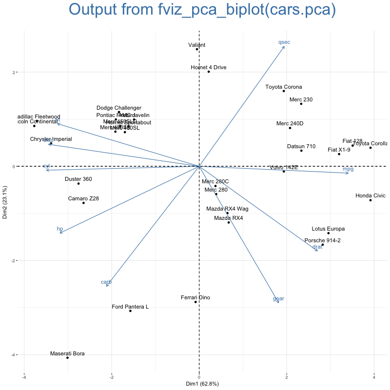
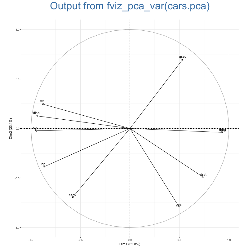
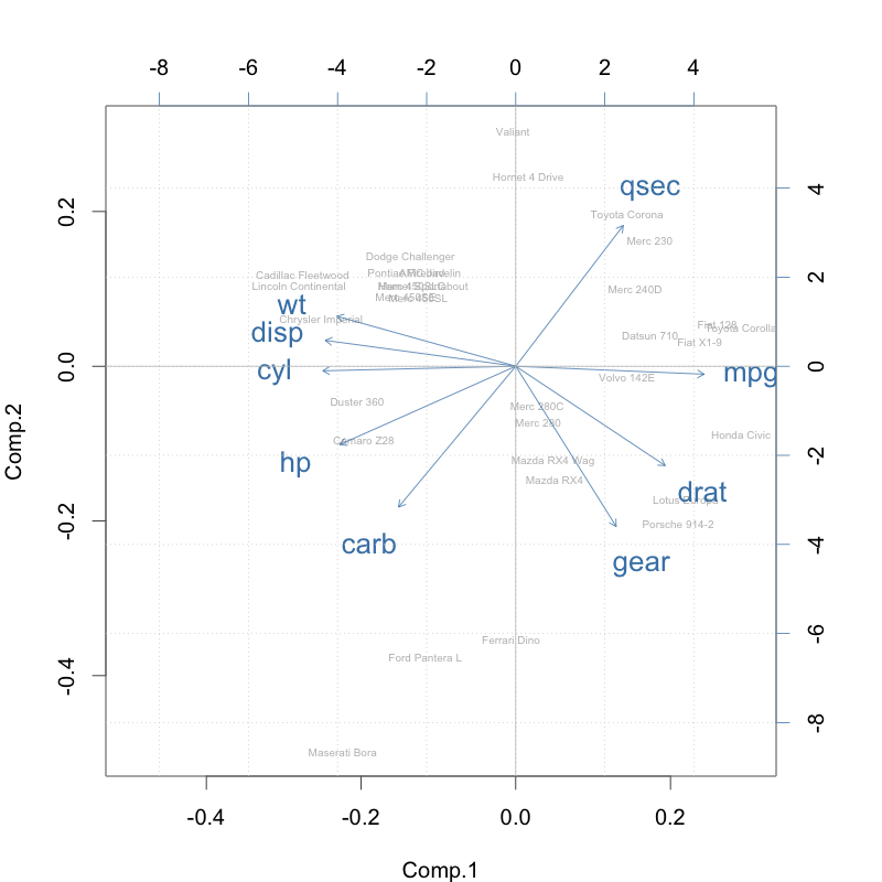
Geometry of loadings - plot

 biplot(cars.pca, col = c("gray","steelblue"), cex = c(0.5, 1.3))

PCA scores

Projection of the original dataset on the principal components.
Total of 9 scores available for each observations

head(cars.pca$scores)


                  Comp.1 Comp.2 Comp.3 Comp.4 Comp.5 Comp.6 Comp.7  Comp.8  Comp.9
Mazda RX4           0.67  -1.19  -0.21 -0.128  0.764 -0.127  0.430  0.0033  0.1697
Mazda RX4 Wag       0.65  -0.99   0.11 -0.087  0.667 -0.067  0.456 -0.0575  0.0727
Datsun 710          2.34   0.33  -0.21 -0.110 -0.077 -0.576 -0.392  0.2053 -0.1163
Hornet 4 Drive      0.22   2.01  -0.33 -0.313 -0.248  0.085 -0.034  0.0241  0.1476
Hornet Sportabout  -1.61   0.84  -1.05  0.150 -0.226  0.186  0.059 -0.1548  0.1571
Valiant            -0.05   2.49   0.11 -0.885 -0.128 -0.234 -0.228 -0.1002  0.0043

PCA scores on first two components

Projection of the original dataset on the principal components
Scores on the first two components

head(cars.pca$scores[, 1:2])

# First two PC scores of first 6 observations
                  Comp.1 Comp.2
Mazda RX4           0.67  -1.19
Mazda RX4 Wag       0.65  -0.99
Datsun 710          2.34   0.33
Hornet 4 Drive      0.22   2.01
Hornet Sportabout  -1.61   0.84
Valiant            -0.05   2.49

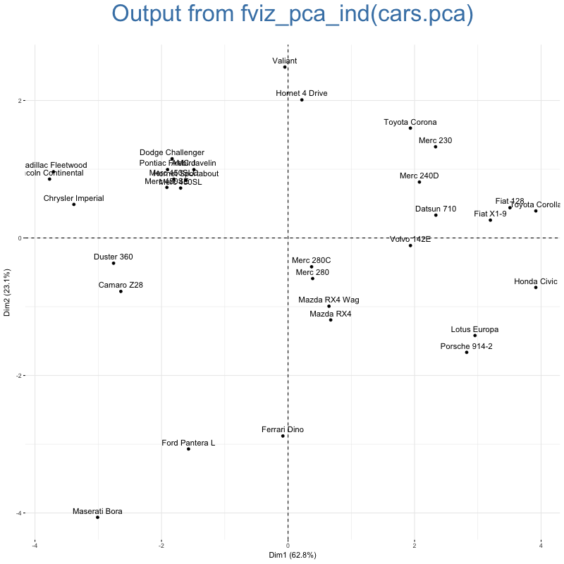
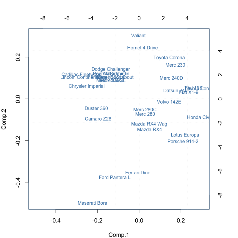
Calculating, visualizing and intrepreting scores

biplot(cars.pca, col = c("steelblue", "white"), cex = c(0.8, 0.01))

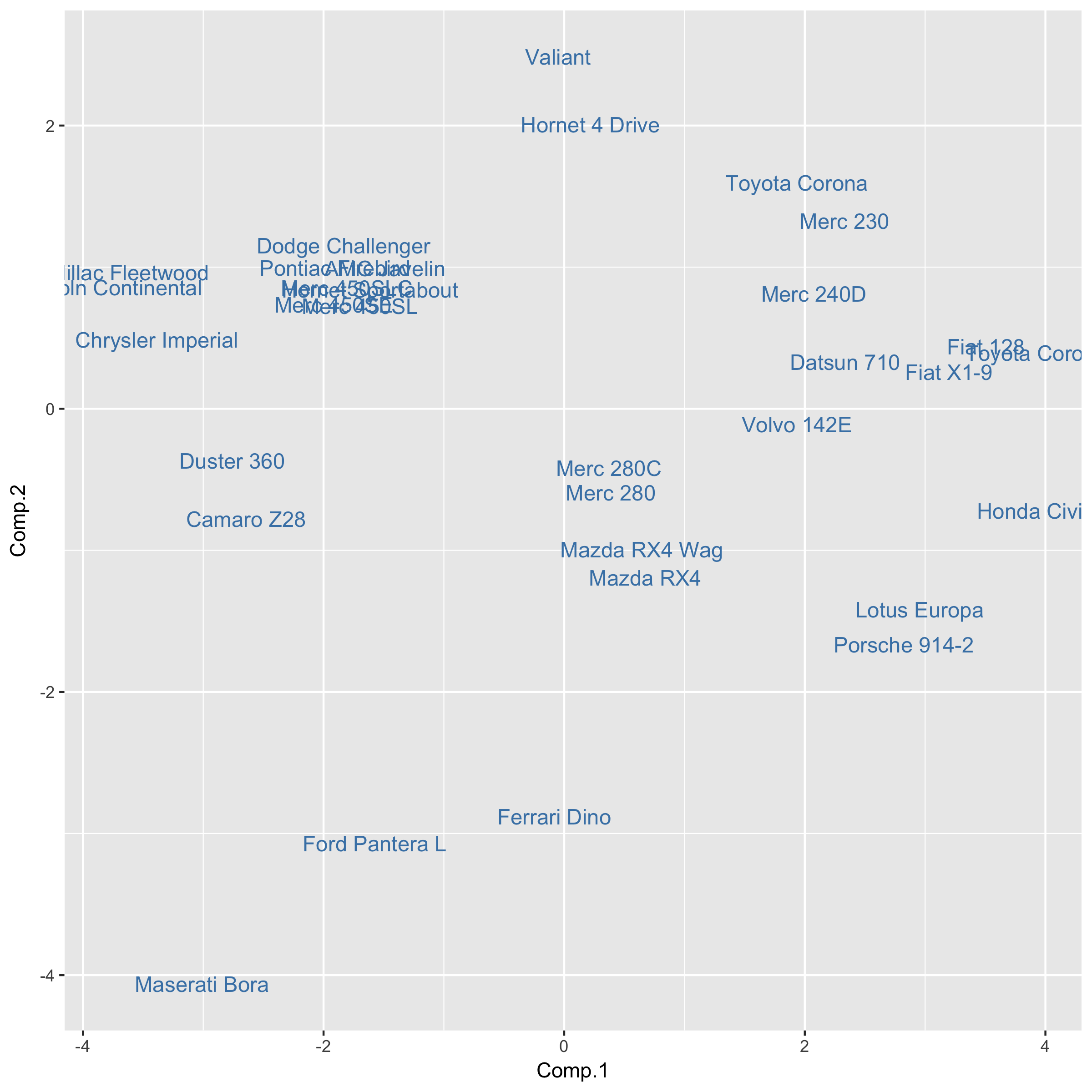
Plotting scores using ggplot

scores <- data.frame(cars.pca$scores)
ggplot(data = scores, aes(x = Comp.1, y = Comp.2, label = rownames(scores))) + 
       geom_text(size = 4, col = "steelblue")

ggplot score

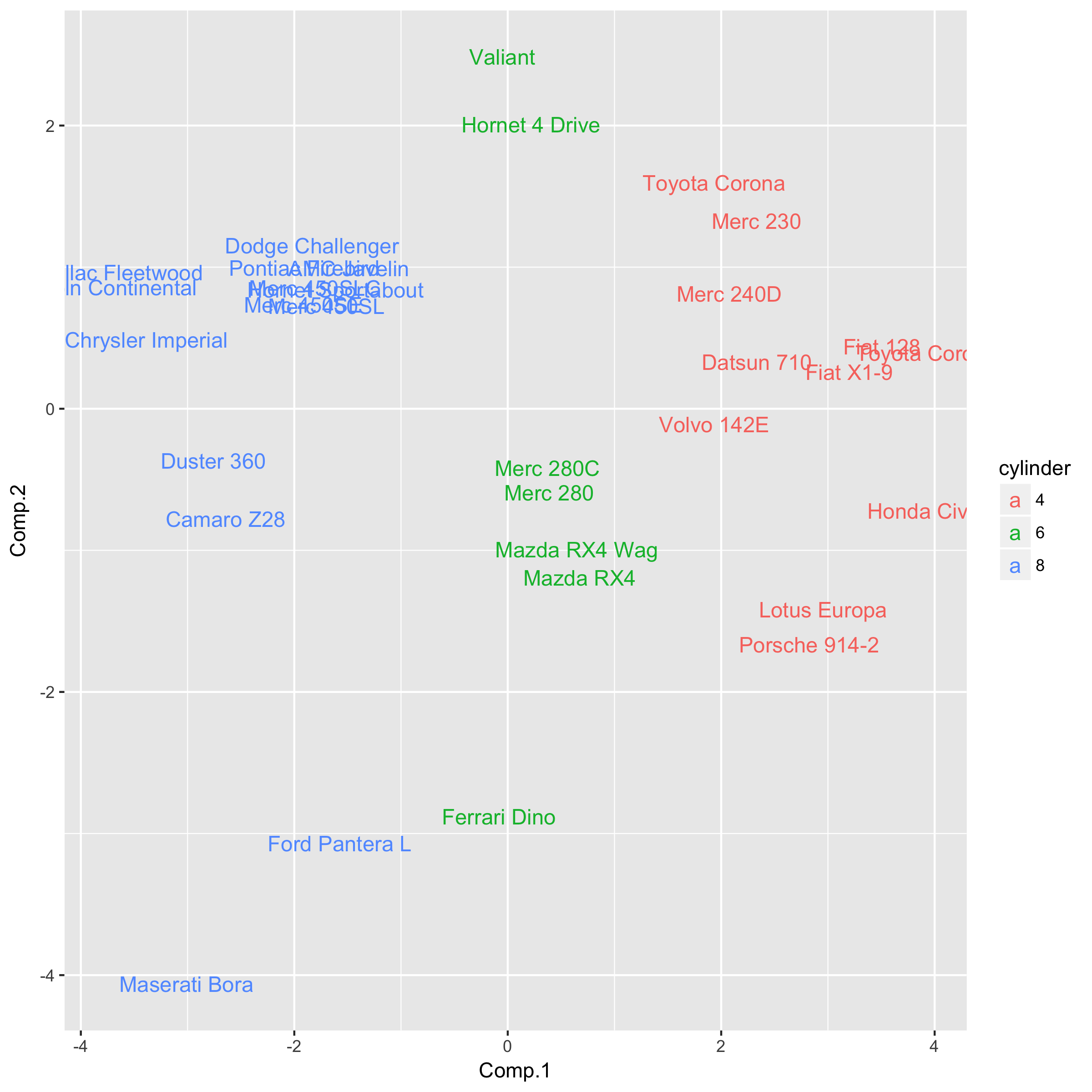
Plotting and coloring scores using ggplot

cylinder <- factor(mtcars$cyl)
ggplot(data = scores, aes(x = Comp.1, y = Comp.2, label = rownames(scores), 
       color = cylinder)) + geom_text(size = 4)

ggplot score colors

Using the factoextra library

fviz_pca_biplot()
fviz_pca_ind()
fviz_pca_var()

Let's practice these functions!

Multivariate Probability Distributions in R