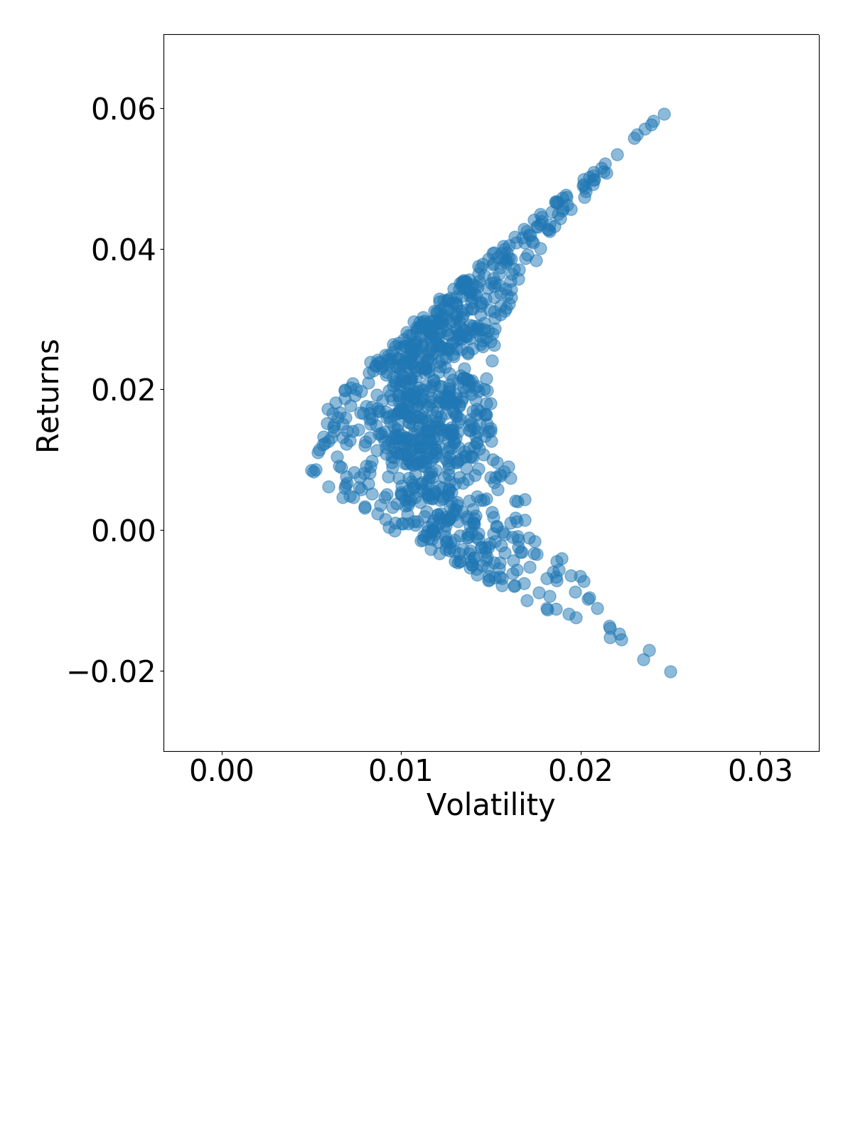
Modern portfolio theory (MPT); efficient frontiers

Machine Learning for Finance in Python

Nathan George

Data Science Professor

efficient frontier

Joining data

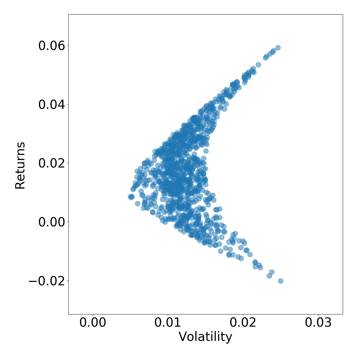
stocks = ['AMD', 'CHK', 'QQQ']
full_df = pd.concat([amd_df, chk_df, qqq_df], axis=1).dropna()
full_df.head()

              AMD       CHK        QQQ
Date                                  
1999-03-10  8.690  0.904417  45.479603
1999-03-11  8.500  0.951617  45.702324
1999-03-12  8.250  0.951617  44.588720
1999-03-15  8.155  0.951617  45.880501
1999-03-16  8.500  0.951617  46.281398

# calculate daily returns of stocks
returns_daily = full_df.pct_change()

# resample the full dataframe to monthly timeframe
monthly_df = full_df.resample('BMS').first()

# calculate monthly returns of the stocks
returns_monthly = monthly_df.pct_change().dropna()
print(returns_monthly.tail())

                 AMD       CHK       QQQ
Date                                    
2018-01-01  0.023299  0.002445  0.028022
2018-02-01  0.206740 -0.156098  0.059751
2018-03-01 -0.101887 -0.190751 -0.020719
2018-04-02 -0.199160  0.060714 -0.052971
2018-05-01  0.167891  0.003367  0.046749

Covariances

# daily covariance of stocks (for each monthly period)
covariances = {}
for i in returns_monthly.index:
    rtd_idx = returns_daily.index
    # mask daily returns for each month (and year) & calculate covariance
    mask = (rtd_idx.month == i.month) & (rtd_idx.year == i.year)
    covariances[i] = returns_daily[mask].cov()

print(covariances[i])

          AMD       CHK       QQQ
AMD  0.000257  0.000177  0.000068
CHK  0.000177  0.002057  0.000108
QQQ  0.000068  0.000108  0.000051

Generating portfolio weights

for date in covariances.keys():
    cov = covariances[date]
    for single_portfolio in range(5000):
        weights = np.random.random(3)
        weights /= np.sum(weights)

Calculating returns and volatility

portfolio_returns, portfolio_volatility, portfolio_weights = {},{},{}

# get portfolio performances at each month
for date in covariances.keys():
    cov = covariances[date]
    for single_portfolio in range(5000):
        weights = np.random.random(3)
        weights /= np.sum(weights)

        returns = np.dot(weights, returns_monthly.loc[date])
        volatility = np.sqrt(np.dot(weights.T, np.dot(cov, weights)))

        portfolio_returns.setdefault(date, []).append(returns)
        portfolio_volatility.setdefault(date, []).append(volatility)
        portfolio_weights.setdefault(date, []).append(weights)

Plotting the efficient frontier

date = sorted(covariances.keys())[-1]
# plot efficient frontier
plt.scatter(x=portfolio_volatility[date],
            y=portfolio_returns[date],
            alpha=0.5)
plt.xlabel('Volatility')
plt.ylabel('Returns')
plt.show()

efficient frontier

Calculate MPT portfolios!

Machine Learning for Finance in Python