Visualizing a categorical variable

Analyzing Survey Data in R

Kelly McConville

Assistant Professor of Statistics

NHANES: visualizing race

library(dplyr)
tab_unw <- NHANESraw %>% group_by(Race1) %>%
   summarize(Freq = n()) %>% mutate(Prop = Freq / sum(Freq)) %>%
   arrange(desc(Prop))

tab_unw

# A tibble: 5 x 3
     Race1  Freq      Prop
    <fctr> <int>     <dbl>
 1    White  7393 0.3643128
 2    Black  4640 0.2286503
 3  Mexican  3739 0.1842507
 4    Other  2312 0.1139309
 5 Hispanic  2209 0.1088553

NHANES documentation

NHANES: visualizing race

library(ggplot2)
ggplot(data = tab_unw, mapping = aes(x = Race1, y = Prop)) + 
  geom_col() + 
  coord_flip() + 
  scale_x_discrete(limits = tab_unw$Race1) # Labels layer omitted

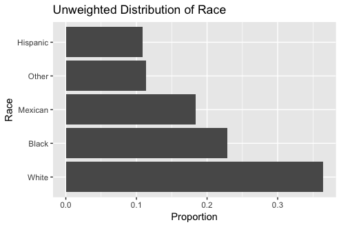
Unweighted barplot of the distribution of race

NHANES: visualizing race

library(ggplot2)
ggplot(data = tab_unw, mapping = aes(x = Race1, y = Prop)) + 
  geom_bar(stat = "identity") + 
  coord_flip() + 
  scale_x_discrete(limits = tab_unw$Race1) # Labels layer omitted

Unweighted barplot of the distribution of race

NHANES: visualizing race

library(ggplot2)
ggplot(data = tab_unw, mapping = aes(x = Race1, y = Prop)) + 
  geom_col() + 
  coord_flip() + 
  scale_x_discrete(limits = tab_unw$Race1) # Labels layer omitted

Unweighted barplot of the distribution of race

NHANES: visualizing race

tab_w <- svytable(~Race1, design = NHANES_design) %>%
   as.data.frame() %>%
   mutate(Prop = Freq / sum(Freq)) %>%
   arrange(desc(Prop))

tab_w

     Race1      Freq       Prop
1    White 193966274 0.63748664
2    Black  37241616 0.12239773
3  Mexican  30719158 0.10096112
4    Other  23389002 0.07686994
5 Hispanic  18951150 0.06228456

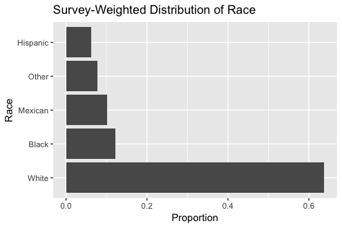
NHANES: visualizing race

ggplot(data = tab_w, mapping = aes(x = Race1, y = Prop)) + 
  geom_col() + 
  coord_flip() + 
  scale_x_discrete(limits = tab_w$Race1) # Labels layer omitted

Survey-weighted barplot of the distribution of race

Let's practice!

Analyzing Survey Data in R