Modeling with linear regression

Analyzing Survey Data in R

Kelly McConville

Assistant Professor of Statistics

Regression line

Scatterplot with trend line of age versus head circumference where transparency represents weights

Regression line

Scatterplot with trend line of age versus head circumference where transparency represents weights. Orange dotted lines to aid with prediction when age is 4 months.

Regression equation

Regression equation is given by:

$$\hat{y} = a + b x$$

Find $a$ and $b$ by minimizing

$$\sum_{i=1}^n w_i (y_i -\hat{y}_i)^2$$

Fitting regression model

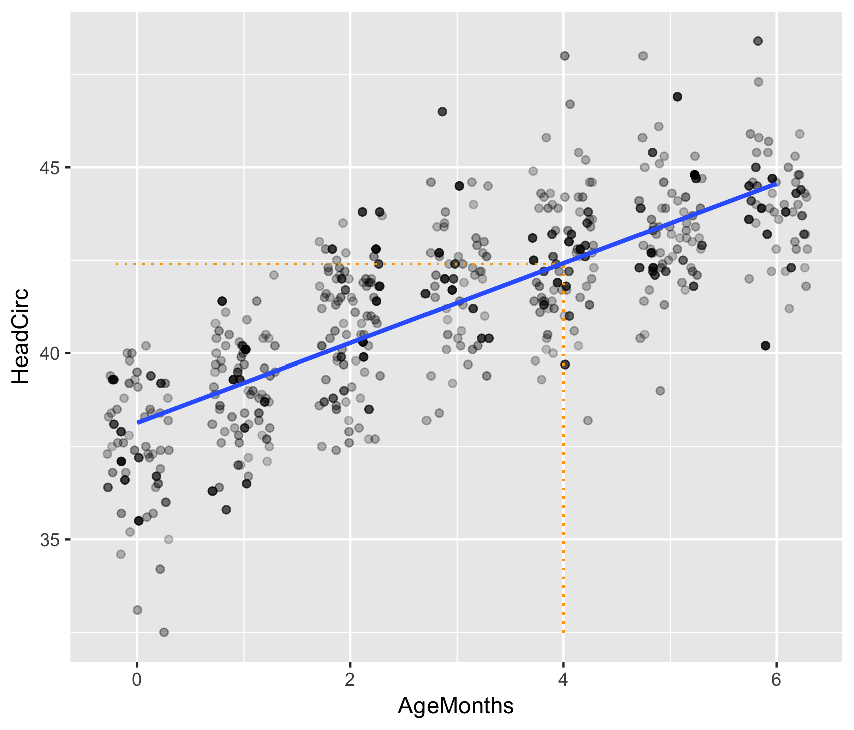
mod <- svyglm(HeadCirc ~ AgeMonths, design = NHANES_design)
summary(mod)

svyglm(formula = HeadCirc ~ AgeMonths, design = NHANES_design)

Survey design:
svydesign(data = NHANESraw, strata = ~SDMVSTRA, id = ~SDMVPSU, 
    nest = TRUE, weights = ~WTMEC4YR)

Coefficients:
            Estimate Std. Error t value Pr(>|t|)    
(Intercept)  38.1376     0.2004   190.3   <2e-16 ***
AgeMonths     1.0708     0.0593    18.1   <2e-16 ***
(Some output omitted)

Linear regression inference

Estimated regression equation is given by:

$$\hat{y} = a + b x$$

True regression equation is given by:

$$E(y) = A + B x$$

$E(y)$ is the average value of $y$ and the variance is sd$(y) = \sigma$.

Linear regression inference

Null Hypothesis: Head size and age are not linearly related (i.e., $B = 0$).

Alternative Hypothesis: Head size and age are linearly related (i.e. $B \neq 0$).

mod <- svyglm(HeadCirc ~ AgeMonths, design = NHANES_design)
summary(mod)

Coefficients:
            Estimate Std. Error t value Pr(>|t|)    
(Intercept)  38.1376     0.2004   190.3   <2e-16 ***
AgeMonths     1.0708     0.0593    18.1   <2e-16 ***
(Some Output Omitted)

Test statistic: $t = \frac{b}{SE}$

Let's practice!

Analyzing Survey Data in R