Introduction

Support Vector Machines in R

Kailash Awati

Instructor

Preliminaries

Objective: gain understanding of how SVMs work; options available in the algorithm and situations in which they work best.
Prerequisites: Intermediate knowledge of R; basic visualization using ggplot().
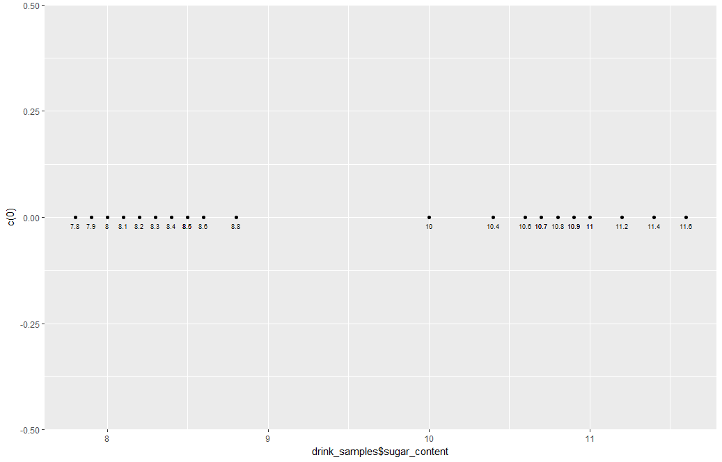
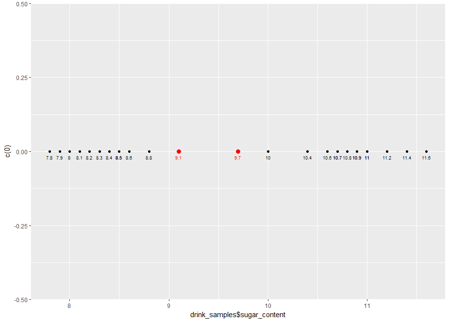
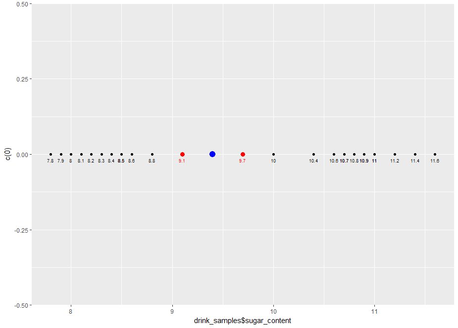
Approach: Start with 1-dimensional example and gradually move on to more complex examples.

Sugar content of soft drinks

Soft drink manufacturer has two versions of flagship brand:
- Choke - sugar content 11g/ 100 ml.
- Choke-R - sugar content 8 g/ 100 ml.
Actual sugar content varies in practice.
Given 25 samples chosen randomly, find a decision rule to determine brand.
First step: visualize data!

Sugar content of soft drinks - visualization code

Data in drink_samples dataframe.

# Specify dataframe, set plot aesthetics in geom_point (note y = 0)
p <- ggplot(drink_samples) +
  geom_point(aes(sugar_content, 0))

# Label each point with sugar content value, adjust text size and location
p <- p +  
  geom_text(aes(sugar_content, 0, label = sugar_content),
            size = 2.5,
            vjust = 2,
            hjust = 0.5)
# Display plot
p

Chapter 1.1 - sugar content clusters

Decision boundaries

Let's pick two points in the interval as candidate boundaries:
- 9.1 g/100 ml
- 9.7 g/100 ml
Classification (decision) rules:
- if (y < 9.1) then "Choke-R" else "Choke"
- if (y < 9.7) then "Choke-R" else "Choke"
Let's visualize them on the plot shown on the previous slide.

Decision boundaries - visualization code

Create a dataframe containing the two decision boundaries.

# Define data frame containing decision boundaries
d_bounds <- data.frame(sep = c(9.1, 9.7))

Decision boundaries - visualization code

Add to plot using geom_point()

# Add decision boundaries to previous plot
p <- p + 
  geom_point(data = d_bounds,
             aes(sep, 0),
             color = "red",
             size = 3) +
  geom_text(data = d_bounds,
            aes(sep, 0, label = sep),
            size = 2.5,
            vjust = 2,
            hjust = 0.5,
            color = "red") 
# Display plot
p

Chapter 1.1 - sugar content clusters with example decision boundaries

Maximum margin separator

The best decision boundary is one that maximizes the margin: maximal margin separator
Maximal margin separator lies halfway between the two clusters.
Visualize the maximal margin separator.

# Create data frame with maximal margin separator
mm_sep <- data.frame(sep = c((8.8 + 10) / 2))

# Add mm boundary to previous plot
p <- p + 
  geom_point(data = mm_sep, 
             aes(sep, 0), 
             color = "blue", 
             size = 4)  
# Display plot
p

Chapter 1.1 - maximal margin separator

Time to practice!

Support Vector Machines in R