Simple feature geometry and tidycensus

Analyzing US Census Data in R

Kyle Walker

Instructor

The geometry = TRUE argument

geometry = TRUE is available for the following geographies:
- "state"
- "county"
- "tract"
- "block group"
- "block"
- "zcta" (also "zip code tabulation area")

Getting simple feature geometry

library(tidycensus)
library(tidyverse)
library(sf)

cook_value <- get_acs(geography = "tract", state = "IL", 
                      county = "Cook", 
                      variables = "B25077_001", 
                      geometry = TRUE)

Simple feature geometry

head(cook_value, 3)

Simple feature collection with 3 features and 5 fields
geometry type:  MULTIPOLYGON
dimension:      XY
bbox:           xmin: -87.68465 ymin: 42.01232 xmax: -87.66434 ymax: 42.02297
epsg (SRID):    4269
proj4string:    +proj=longlat +datum=NAD83 +no_defs
        GEOID                                       NAME   variable
1 17031010100    Census Tract 101, Cook County, Illinois B25077_001
2 17031010201 Census Tract 102.01, Cook County, Illinois B25077_001
3 17031010202 Census Tract 102.02, Cook County, Illinois B25077_001
  estimate   moe                       geometry
1   230700 62332 MULTIPOLYGON (((-87.6772 42...
2   151100 19099 MULTIPOLYGON (((-87.68465 4...
3   133300 84063 MULTIPOLYGON (((-87.67685 4...

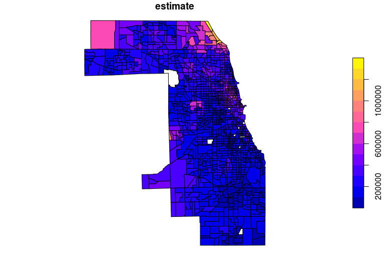
Plotting tidycensus geometry

plot(cook_value["estimate"])

basic cook county plot

Joining tigris and tidycensus data

library(tigris)

idaho_income <- get_acs(geography = "school district (unified)", 
                        variables = "B19013_001", 
                        state = "ID")

idaho_school <- school_districts(state = "ID", 
                                 type = "unified", 
                                 class = "sf")

id_school_joined <- left_join(idaho_school, 
                              idaho_income, 
                              by = "GEOID")

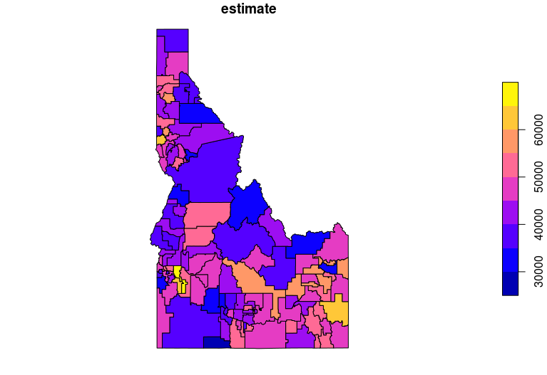
Joining tigris and tidycensus data

plot(id_school_joined["estimate"])

Income by school district in Idaho

Shifting Alaska and Hawaii geometry

state_value <- get_acs(geography = "state", 
                       variables = "B25077_001", 
                       survey = "acs1", 
                       geometry = TRUE, 
                       shift_geo = TRUE)

plot(state_value["estimate"])

Plot of shift_geo

Let's practice!

Analyzing US Census Data in R