Cartographic workflows with tigris and tidycensus

Analyzing US Census Data in R

Kyle Walker

Instructor

Education dot map

Generating random dots with sf

Key function for random point generation in sf: st_sample()

dc_dots <- map(c("White", "Black", "Hispanic", "Asian"), function(group) {
  dc_race %>%
    filter(variable == group) %>%
    st_sample(., size = .$value / 100) %>%
    st_sf() %>%
    mutate(group = group) 
}) %>%
  reduce(rbind)

Considerations for random dot generation

For faster plotting:

dc_dots <- dc_dots %>%
  group_by(group) %>%
  summarize()

For more accurate visualizations:

dc_dots_shuffle <- sample_frac(dc_dots, size = 1)

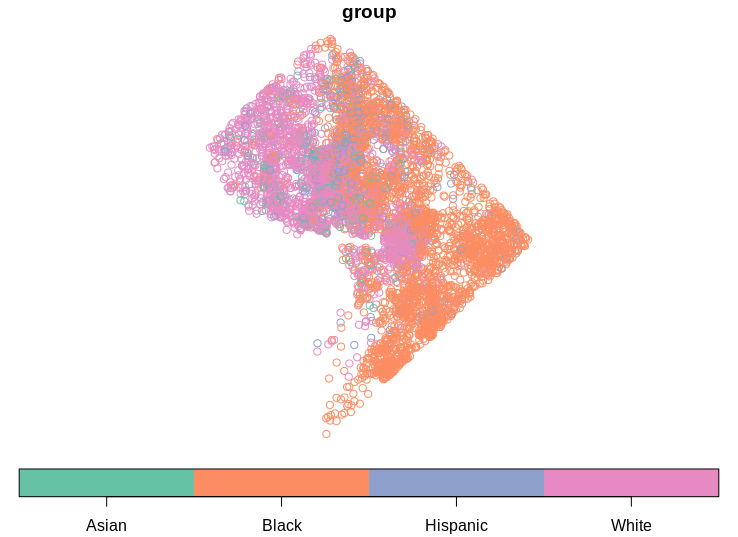
Basic dot-density mapping with sf

plot(dc_dots_shuffle, key.pos = 1)

Basic dot density map

Ancillary data with tigris

options(tigris_class = "sf")

dc_roads <- roads("DC", "District of Columbia") %>%
  filter(RTTYP %in% c("I", "S", "U"))

dc_water <- area_water("DC", "District of Columbia")

dc_boundary <- counties("DC", cb = TRUE)

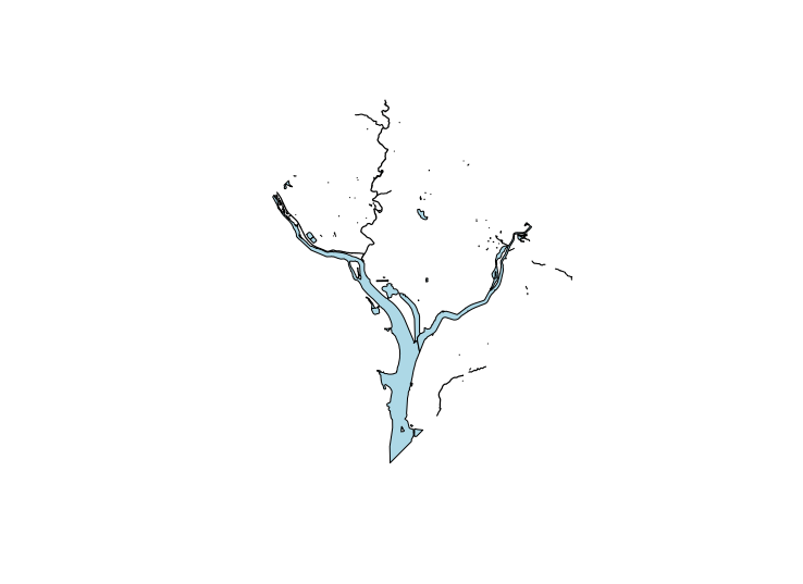
Ancillary data with tigris

plot(dc_water$geometry, col = "lightblue")

DC water plot

Dot-density mapping with ggplot2

ggplot() + 
  geom_sf(data = dc_boundary, color = NA, fill = "white") + 
  geom_sf(data = dc_dots, aes(color = group, fill = group), size = 0.1) + 
  geom_sf(data = dc_water, color = "lightblue", fill = "lightblue") + 
  geom_sf(data = dc_roads, color = "grey") + 
  coord_sf(crs = 26918, datum = NA) + 
  scale_color_brewer(palette = "Set1", guide = FALSE) +
  scale_fill_brewer(palette = "Set1") +
  labs(title = "The racial geography of Washington, DC", 
       subtitle = "2010 decennial U.S. Census", 
       fill = "", 
       caption = "1 dot = approximately 100 people.\nData acquired with 
                  the R tidycensus and tigris packages.")

Final dot density map

Considerations for dot-density mapping

Be mindful of ways dot-density maps can be misinterpreted
Choose qualitative colors wisely
Take care when selecting ancillary layers

Let's practice!

Analyzing US Census Data in R