Evaluating the fit of many models

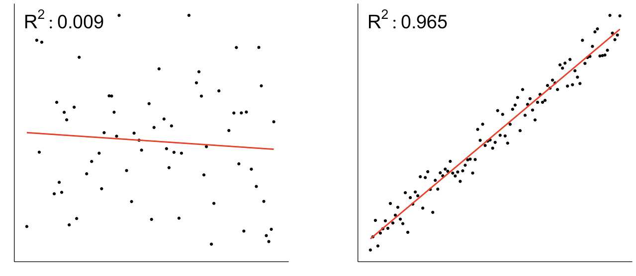
Machine Learning in the Tidyverse

Dmitriy (Dima) Gorenshteyn

Lead Data Scientist, Memorial Sloan Kettering Cancer Center

The fit of our models

$$ R^2 = \frac{\%\ variation\ explained\ by\ the\ model}{\%\ total\ variation\ in\ the\ data} $$

The fit of our models

Glance across your models

model_perf <- gap_models %>% 
  mutate(coef = map(model, ~glance(.x))) %>%
  unnest(coef)

model_perf

# A tibble: 77 x 14
   country  data  model r.squared adj.r.squared sigma statistic   ...
   <fct>    <lis> <lis>     <dbl>         <dbl> <dbl>     <dbl>   ...
 1 Algeria  <tib… <S3:.       0.952        0.951   2.18    996    ...
 2 Argenti. <tib… <S3:.       0.984        0.984   0.431  3137    ...
 3 Austral. <tib… <S3:.       0.983        0.983   0.511  2905    ...
 4 Austria  <tib… <S3:.       0.987        0.986   0.438  3702    ...
 5 Banglad. <tib… <S3:.       0.949        0.947   1.83    921    ...
 6 Belgium. <tib… <S3:.       0.990        0.990   0.331  5094    ...
 # ... with 71 more rows

model_perf %>% 
  slice_max(r.squared, n = 2)

# A tibble: 2 x 14
  country data  model r.squared adj.r.squared sigma statistic
  <fct>   <lis> <lis>     <dbl>         <dbl> <dbl>     <dbl>
1 Canada  <tib… <S3:.     0.995         0.995 0.231    10117
2 Italy   <tib… <S3:.     0.997         0.997 0.226    15665

model_perf %>% 
  slice_min(r.squared, n = 2)

# A tibble: 2 x 14
  country data  model r.squared adj.r.squared sigma statistic
  <fct>   <lis> <lis>     <dbl>         <dbl> <dbl>     <dbl>
1 Botswa~ <tib… <S3:.   0.0136       -0.00608  5.11     0.692
2 Lesotho <tib… <S3:.   0.00296      -0.0170   5.32     0.148

Let's practice!

Machine Learning in the Tidyverse