Visually inspect the fit of your models

Machine Learning in the Tidyverse

Dmitriy (Dima) Gorenshteyn

Lead Data Scientist, Memorial Sloan Kettering Cancer Center

Building augmented datframes

augmented_models <- gap_models %>% 
                    mutate(augmented = map(model, ~augment(.x))) %>%
                    unnest(augmented)

augmented_models

# A tibble: 4,004 x 10
   country life_expectancy  year .fitted .se.fit .resid   .hat .sigma 
   <fct>             <dbl> <int>   <dbl>   <dbl>  <dbl>  <dbl>  <dbl> 
 1 Algeria            47.5  1960    47.8   0.595 -0.266 0.0747   2.20 
 2 Algeria            48.0  1961    48.4   0.578 -0.381 0.0705   2.20 
 3 Algeria            48.6  1962    49.0   0.561 -0.486 0.0664   2.20 
 4 Algeria            49.1  1963    49.7   0.544 -0.600 0.0625   2.20 
 5 Algeria            49.6  1964    50.3   0.527 -0.725 0.0587   2.20 
 6 Algeria            50.1  1965    50.9   0.511 -0.850 0.0551   2.20

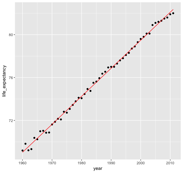
Model for Italy $R^2: 0.99$

augmented_model %>% filter(country == "Italy") %>% 
  ggplot(aes(x = year, y = life_expectancy)) + 
  geom_point() +
  geom_line(aes(y = .fitted), color = "red")

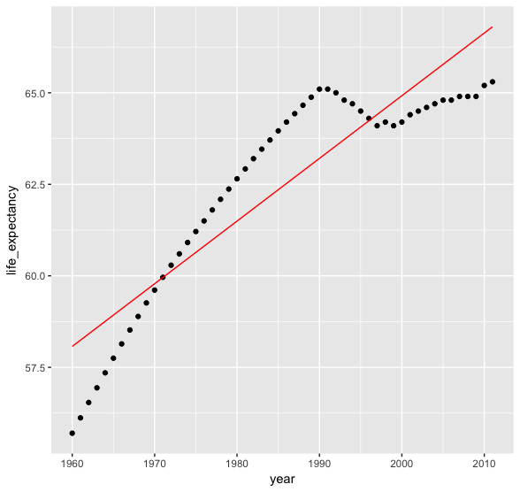
Model for Fiji $R^2: 0.82$

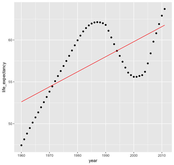
Model for Kenya $R^2: 0.42$

Let's practice!

Machine Learning in the Tidyverse