Exploring coefficients across models

Machine Learning in the Tidyverse

Dmitriy (Dima) Gorenshteyn

Lead Data Scientist, <Memorial Sloan Kettering Cancer Center

77 models

gap_nested <- gapminder %>% 
              group_by(country) %>%
              nest()
gap_models <- gap_nested %>%
              mutate(
                  model = map(data, ~lm(life_expectancy~year, data = .x)))

gap_models

# A tibble: 77 x 3
   country    data              model   
   <fct>      <list>            <list>  
 1 Algeria    <tibble [52 × 6]> <S3: lm>
 2 Argentina  <tibble [52 × 6]> <S3: lm>
 3 Australia  <tibble [52 × 6]> <S3: lm>
 4 Austria    <tibble [52 × 6]> <S3: lm>
 5 Bangladesh <tibble [52 × 6]> <S3: lm>

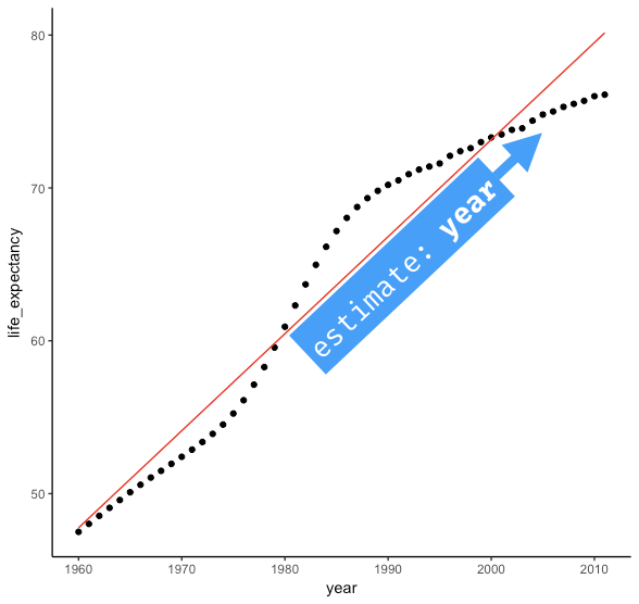
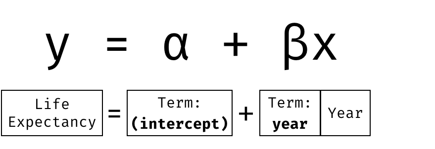
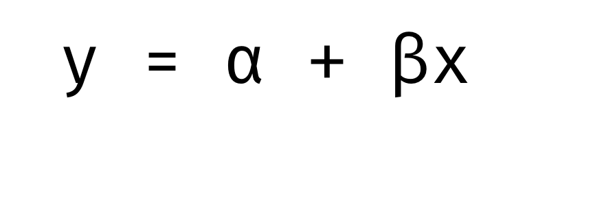
Regression coefficients

tidy(gap_models$model[[1]])

         term      estimate     ...
1 (Intercept) -1196.5647772     ...
2        year     0.6348625     ...

Coefficients of multiple models

gap_models %>% 
  mutate(coef = map(model, ~tidy(.x))) %>%
  unnest(coef)

# A tibble: 154 x 6
   country    term         estimate std.error statistic   p.value
   <fct>      <chr>           <dbl>     <dbl>     <dbl>     <dbl>
 1 Algeria    (Intercept) -1197      39.9         -30.0  1.32e-33
 2 Algeria    year            0.635   0.0201       31.6  1.11e-34
 3 Argentina  (Intercept) - 372       7.91        -47.0  4.66e-43
 4 Argentina  year            0.223   0.00398      56.0  8.78e-47
 5 Australia  (Intercept) - 429       9.37        -45.8  1.71e-42
 6 Australia  year            0.254   0.00472      53.9  5.83e-46

Let's practice!

Machine Learning in the Tidyverse