Simulation testing solution

Supply Chain Analytics in Python

Aaren Stubberfield

Supply Chain Analytics Mgr.

Caution

Problems that take a long time to solve should not be used with LP or IP

caution image, man slipping

Overall concept

General Concept:

Add random noise to key inputs you choose
Solve the model repeatedly
Observe the distribution

Why we might try

Why:

Inputs are often estimates. There is a risk that they are inaccurate.
Earlier Sensitivity Analysis only looked at changing one input at a time.

Context

Context - Glass Company - Resource Planning:

Resource	Prod. A	Prod. B	Prod. C
Profit $US	$500	$450	$600

Constraints:

There are demand, production capacity, and warehouse Capacity constraints

Risks:

Estimates of profits may be inaccurate

# Initialize Class, & Define Variables
model = LpProblem("Max Glass Co. Profits", LpMaximize)
A = LpVariable('A', lowBound=0)
B = LpVariable('B', lowBound=0)
C = LpVariable('C', lowBound=0)

# Define Objective Function
model += 500 * A + 450 * B + 600 * C

# Define Constraints & Solve
model += 6 * A + 5 * B + 8 * C <= 60
model += 10.5 * A + 20 * B + 10 * C <= 150
model += A  <= 8
model.solve()

Code example - step 2

a, b, c = normalvariate(0,25), 
          normalvariate(0,25),
          normalvariate(0,25)

# Define Objective Function
model += (500+a)*A + (450+b)*B + (600+c)*C

# Initialize Class, & Define Variables
model = LpProblem("Max Glass Co. Profits", 
                   LpMaximize)

A = LpVariable('A', lowBound=0)
B = LpVariable('B', lowBound=0)
C = LpVariable('C', lowBound=0)
a, b, c = normalvariate(0,25), 
          normalvariate(0,25), 
          normalvariate(0,25)
# Define Objective Function
model += (500+a)*A + (450+b)*B + (600+c)*C

# Define Constraints & Solve
model += 6 * A + 5 * B + 8 * C <= 60
model += 10.5 * A + 20 * B + 10 * C <= 150
model += A  <= 8
model.solve()

def run_pulp_model():
    # Initialize Class
    model = LpProblem("Max Glass Co. Profits", LpMaximize)
    A = LpVariable('A', lowBound=0)
    B = LpVariable('B', lowBound=0)
    C = LpVariable('C', lowBound=0)
    a, b, c = normalvariate(0,25), normalvariate(0,25), normalvariate(0,25)

    # Define Objective Function
    model += (500+a)*A + (450+b)*B + (600+c)*C

    # Define Constraints & Solve
    model += 6 * A + 5 * B + 8 * C <= 60
    model += 10.5 * A + 20 * B + 10 * C <= 150
    model += A  <= 8
    model.solve()
    o = {'A':A.varValue, 'B':B.varValue, 'C':C.varValue, 'Obj':value(model.objective)}
    return(o)

Code example - step 4

def run_pulp_model():
    # Initialize Class
    model = LpProblem("Max Glass Co. Profits",
                       LpMaximize)
    A = LpVariable('A', lowBound=0)
    B = LpVariable('B', lowBound=0)
    C = LpVariable('C', lowBound=0)
    a, b, c = normalvariate(0,25), 
              normalvariate(0,25),
              normalvariate(0,25)

    # Define Objective Function
    model += (500+a)*A + (450+b)*B + 
             (600+c)*C

    # Define Constraints & Solve
    model += 6 * A + 5 * B + 8 * C <= 60
    model += 10.5 * A + 20 * B + 10 * C <= 150
    model += A  <= 8
    model.solve()
    o = {'A':A.varValue, 'B':B.varValue, 
         'C':C.varValue, 
         'Obj':value(model.objective)}
    return(o)

for i in range(100):
    output.append(run_pulp_model())
df = pd.DataFrame(output)

Code example - step 5

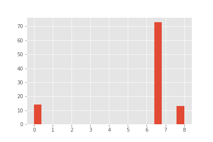
print(df['A'].value_counts())
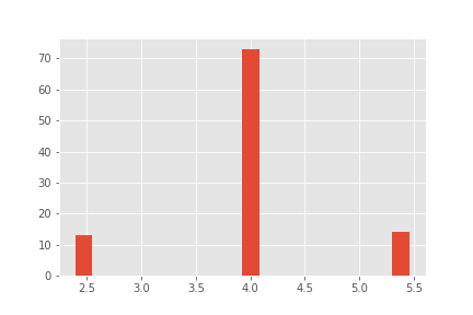
print(df['B'].value_counts())
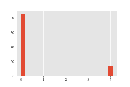
print(df['C'].value_counts())

Output: (results may be different)

6.666667    73
0.000000    14
8.000000    13
Name: A, dtype: int64

4.000000    73
5.454546    14
2.400000    13
Name: B, dtype: int64
0.000000    86
4.090909    14
Name: C, dtype: int64

Visualize as histogram

Product A: histogram of product a, b, c, and objective

Product B: histogram of product b

Product C: histogram of product c

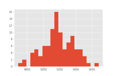
Objective Values: histogram of objective values

Summary

Should not be used on problems that take a long time to solve
Benefits
- View how optimal results change as model inputs change
Steps
1. Start with standard PuLP model code
2. Add noise to key inputs using Python's normalvariate
3. Wrap PuLP model code in a function that returns the model's output
4. Create loop to call newly created function and store results in DataFrame
5. Visualize results DataFrame

Try it out!

Supply Chain Analytics in Python