Capacitated plant location - case study P4

Supply Chain Analytics in Python

Aaren Stubberfield

Supply Chain Analytics Mgr., Ingredion

Simulation vs. sensitivity analysis

With Sensitivity Analysis:

Observe how changes in demand and costs affect production:
- Where should production be added?
- Does production move to a different region.
- Which regions have stable production quantities?
Observe multiple changes at once vs. one at a time with sensitivity analysis

Simulation modeling

We can apply simulation testing to our Capacitated Plant Location Model

Possible inputs for adding noise

Demand
Variable costs
Fixed costs
Capacity

# Initialize Class
model = LpProblem(
            "Capacitated Plant Location Model",
             LpMinimize)

# Define Decision Variables
loc = ['A', 'B', 'C', 'D', 'E']
size = ['Low_Cap','High_Cap']
x = LpVariable.dicts(
       "production_", 
       [(i,j) for i in loc for j in loc],
       lowBound=0, upBound=None, cat='Continuous')
y = LpVariable.dicts(
      "plant_", [(i,s)for s in size for i in loc], 
       cat='Binary')

# Define Objective Function
model +=(lpSum([fix_cost.loc[i,s]*y[(i,s)]
               for s in size for i in loc])
       + lpSum([var_cost.loc[i,j]*x[(i,j)]
                for i in loc for j in loc]))

# Define the Constraints
for j in loc: model += 
  lpSum([x[(i, j)] for i in loc]) == demand.loc[
                                          j,'Dmd']
for i in loc: model += 
  lpSum([x[(i, j)] for j in loc]) <= lpSum(
                            [cap.loc[i,s]*y[(i,s)]
                             for s in size])
# Solve
model.solve()
print(LpStatus[model.status])

Objective:

model += (lpSum([fix_cost.loc[i,s]*y[(i,s)] for s in size for i in loc])
          + lpSum([(var_cost.loc[i,j] + normalvariate(0.5, 0.5))*x[(i,j)] 
                   for i in loc for j in loc]))

Total Demand:

for j in loc:
    rd = normalvariate(0, demand.loc[j,'Dmd']*.05)
    model += lpSum([x[(i,j)] for i in loc]) == (demand.loc[j,'Dmd']+rd)

Code example - step 3

def run_pulp_model(fix_cost, var_cost, demand,
                   cap):
    # Initialize Class
    model = LpProblem(
              "Capacitated Plant Location Model", 
               LpMinimize)

    # Define Decision Variables
    loc = ['A', 'B', 'C', 'D', 'E']
    size = ['Low_Cap','High_Cap']
    x = LpVariable.dicts(
                "production_", 
                [(i,j) for i in loc for j in loc],
                lowBound=0, upBound=None,
                cat='Continuous')

    y = LpVariable.dicts(
               "plant_", 
               [(i,s) for s in size for i in loc], 
                cat='Binary')
    # Define the Constraints
    for j in loc: rd = normalvariate(
                       0, demand.loc[j,'Dmd']*.05)
        model += lpSum(
         [x[(i,j)] for i in loc]) == (
                           demand.loc[j,'Dmd']+rd)
    for i in loc: model += 
      lpSum([x[(i,j)] for j in loc]) \
        <= lpSum([cap.loc[i,s]*y[(i,s)] 
            for s in size])

    # Solve
    model.solve()
    o = {}
    for i in loc:
        o[i] = value(lpSum([x[(i, j)] for j in loc]))
    o['Obj'] = value(model.objective)
    return(o)

for i in range(100):
    output.append(run_pulp_model(fix_cost, var_cost, demand, cap))
df = pd.DataFrame(output)

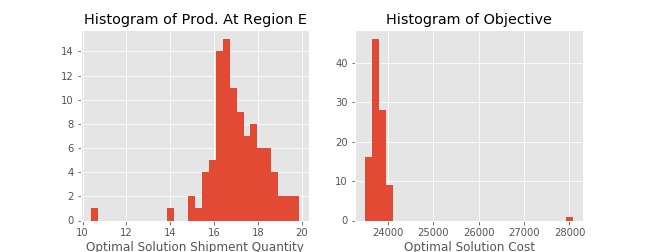
Results

import matplotlib.pyplot as plt
plt.title('Histogram of Prod. At Region E')
plt.hist(df['E'])
plt.show()

histogram results of E region and objective

Summary

Capacitated Plant Model

Simulation vs. sensitivity analysis
Stepped through code example

Try it out!

Supply Chain Analytics in Python