GARCH models: The way forward
GARCH Models in R

Kris Boudt
Professor of finance and econometrics
Inventors of GARCH models
Robert Engle
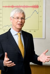
Tim Bollerslev

Notation (i)
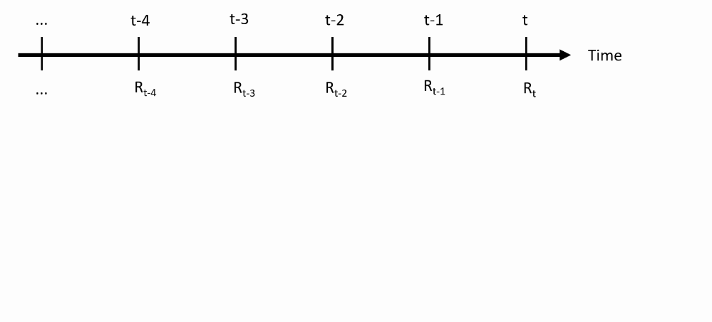
- Input: Time series of returns
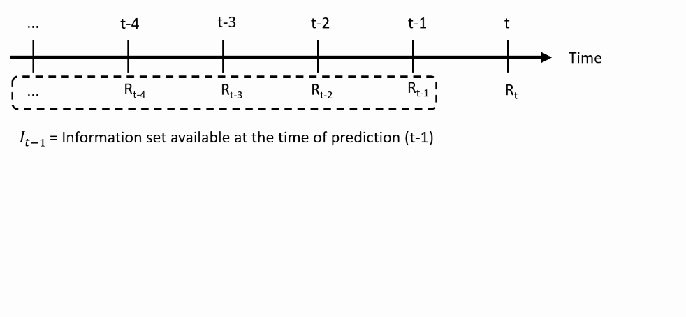
Notation (ii)
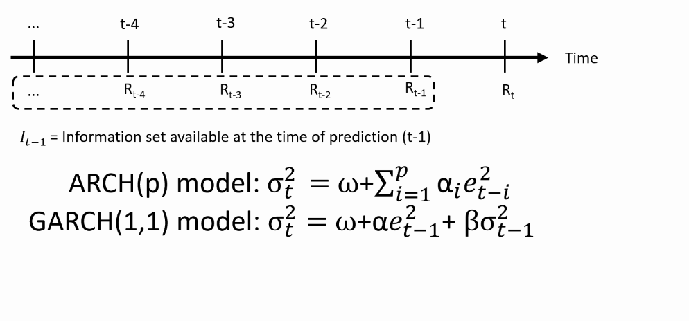
- At time $t-1$, you make the prediction about the the future return $R_t$, using the information set available at time $t-1$:
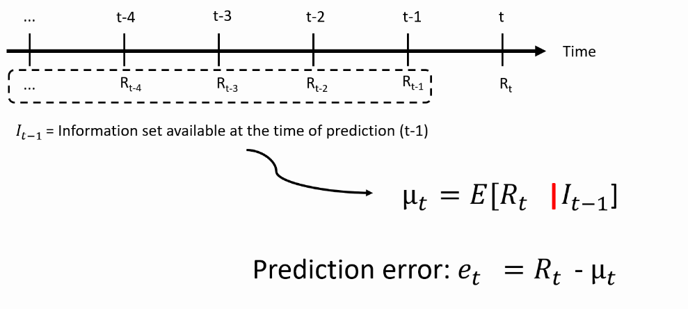
Notation (iii)
- Predicting the mean return: what is the best possible prediction of the actual return?
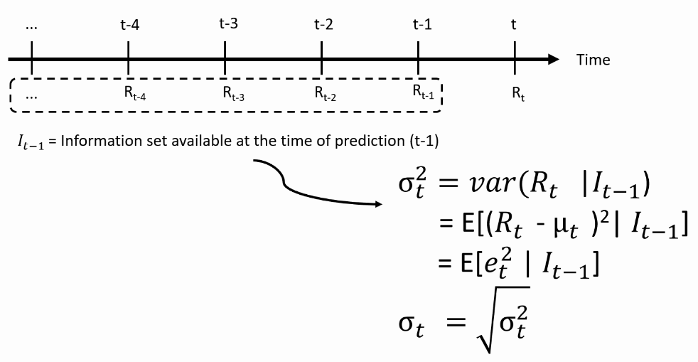
Notation (iv)
- We then predict the variance: how far off the return can be from its mean?
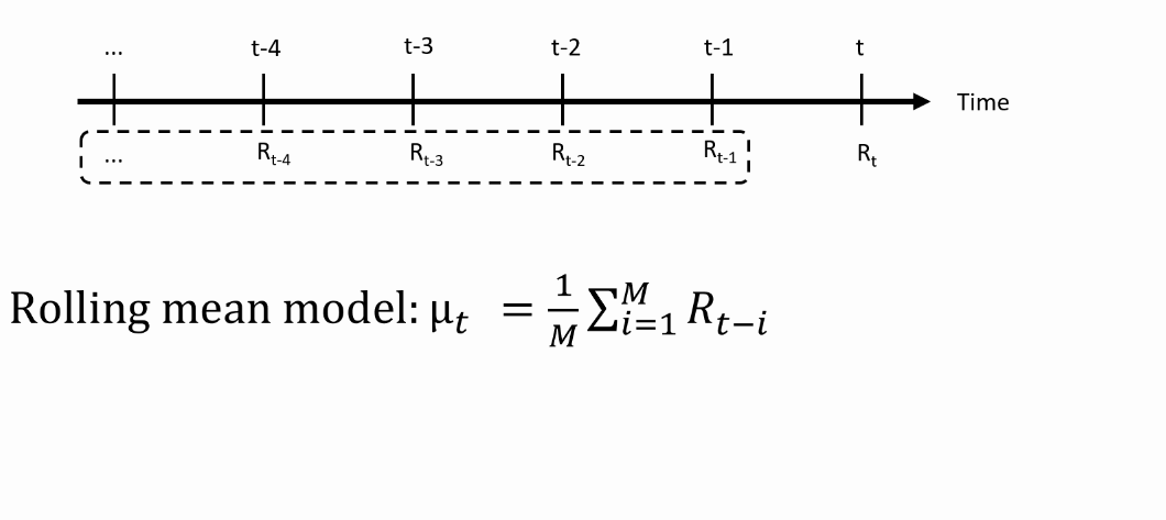
From theory to practice: Models for the mean
- We need an equation that maps the past returns into a prediction of the mean
For AR(MA) models for the mean, see Datacamp course on time series analysis.
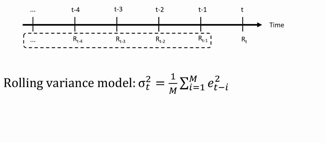
From theory to practice: Models for the variance
- We need an equation that maps the past returns into predictions of the variance
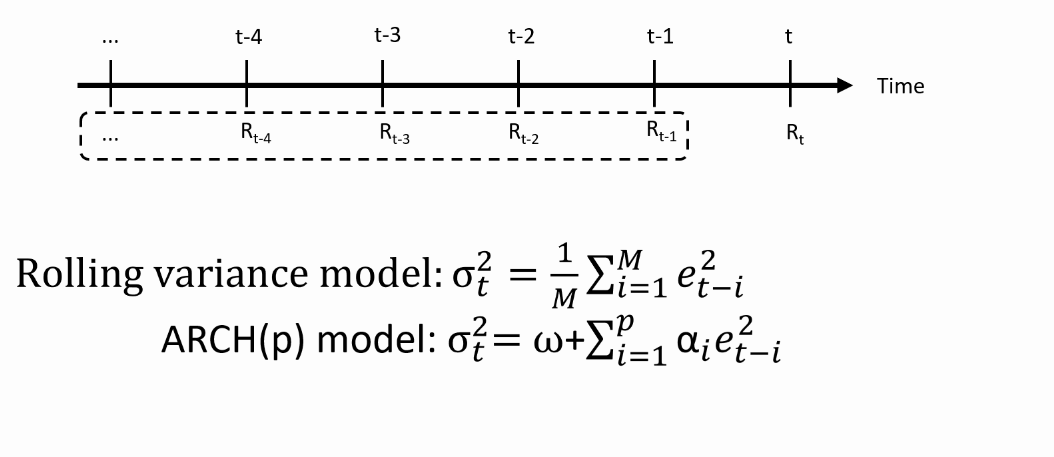
ARCH(p) model: Autoregressive Conditional Heteroscedasticity
- We need an equation that maps the past returns into predictions of the variance
GARCH(1,1) model: Generalized ARCH
- We need an equation that maps the past returns into predictions of the variance