Do the GARCH predictions fit will with the observed returns?

GARCH Models in R

Kris Boudt

Professor of finance and econometrics

Evaluation criterion

Depends on what you want to evaluate
- the predicted mean
- the predicted variance
- the predicted distribution of the returns

1) Goodness of fit for the mean prediction

Based on the estimated GARCH model, we have:

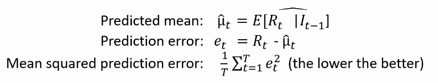
Implementation

e <- residuals(tgarchfit) 
mean(e ^ 2)

2) Goodness of fit for the variance prediction

The GARCH model leads to:

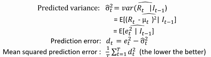
Implementation

e <- residuals(tgarchfit)
d <- e ^ 2 - sigma(tgarchfit) ^ 2 
mean(d ^ 2)

Example for EUR/USD returns

tgarchspec <- ugarchspec(mean.model = list(armaOrder = c(0, 0)),
   variance.model = list(model = "sGARCH", variance.targeting = TRUE),
   distribution.model = "std")
tgarchfit <- ugarchfit(data = EURUSDret, spec = tgarchspec)

# Compute mean squared prediction error for the mean
e <- residuals(tgarchfit) ^ 2
mean(e ^ 2) # 3.836205e-05
# Compute mean squared prediction error for the variance
d <- e ^ 2 - sigma(tgarchfit) ^ 2
mean(d ^ 2) # 5.662366e-09

3) Goodness of fit for the distribution

The GARCH model provides a predicted density for all the returns in the sample
- The higher the density, the more likely the return is under the estimated GARCH model
- The likelihood of the sample is based on the product of all these densities. It measures how likely it is to that the observed returns come from the estimated GARCH model
- The higher the likelihood, the better the model fits with your data

Example for EUR/USD returns

likelihood(tgarchfit) # returns 18528.58

Analyze by comparing with other models:

# Complex model with many parameters
flexgarchspec <- ugarchspec(mean.model = list(armaOrder = c(1, 0)),
                            variance.model = list(model = "gjrGARCH"),
                            distribution.model = "sstd")
flexgarchfit <- ugarchfit(data = EURUSDret, spec = flexgarchspec)
likelihood(flexgarchfit) # returns 18530.49

Risk of overfitting

Attention: We use an in-sample evaluation approach where the estimation sample and evaluation sample coincides.

Danger of overfitting:

Overfitting consists of choosing overly complex models that provide a good fit for the returns in the estimation sample used but not for the future returns that are outside of the sample.

Solution: Balance goodness of fit with a penalty for the complexity

A GARCH model is parsimonious when it has:
- a high likelihood
- and a relatively low number of parameters

Information criteria

Parsimony is measured information criteria.

information criteria = - likelihood + penalty(number of parameters)

The lower, the better.

Rule of thumb for deciding:
Choose the model with lowest information criterion.

Results information criteria

Method infocriteria() prints the information criteria for various penalties

infocriteria(tgarchfit)

out Akaike -7.468081 Bayes -7.462833 Shibata -7.468083 Hannan-Quinn -7.466241 `

Interpretation requires to compare with the information criteria of other models.

Illustration on the EUR/USD returns

tgarchspec <- ugarchspec(mean.model = list(armaOrder = c(0, 0)),
   variance.model = list(model = "sGARCH", variance.targeting = TRUE),
   distribution.model = "std")
tgarchfit <- ugarchfit(data = EURUSDret, spec = tgarchspec)
length(coef(tgarchfit)) # only 5 parameters
likelihood(tgarchfit)   # equals 18528.58

flexgarchspec <- ugarchspec(mean.model = list(armaOrder = c(1, 0)),
   variance.model = list(model = "gjrGARCH"), distribution.model = "sstd")
flexgarchfit <- ugarchfit(data = EURUSDret, spec = flexgarchspec)
length(coef(flexgarchfit)) # we now have 8 parameters
likelihood(flexgarchfit) #  18530.49: likelihood increased

Which model is most parsimonious for EUR/USD returns?

Higher Likelihood is better. Lower information criteria is better.

infocriteria(tgarchfit) # Simple model

Akaike       -7.468435
Bayes        -7.464499

infocriteria(flexgarchfit) # Complex model

Akaike       -7.467239
Bayes        -7.456742

The simple model has the lowest information criterion and should thus be preferred here.

Result is case-specific: case of MSFT returns

tgarchfit <- ugarchfit(data = msftret, spec = tgarchspec)
flexgarchfit <- ugarchfit(data = msftret, spec = flexgarchspec)
infocriteria(tgarchfit)

Akaike       -5.481895
Bayes        -5.477833

infocriteria(flexgarchfit)

Akaike       -5.489087
Bayes        -5.478255

The complex model has the lowest information criterion and should thus be preferred here.

KISS: Keep it Sophisticatedly Simple

GARCH Models in R