Use only the data that were available at the time of prediction

GARCH Models in R

Kris Boudt

Professor of finance and econometrics

Volatility prediction by applying `sigma()` to `ugarchforecast` object

garchspec <- ugarchspec(mean.model = list(armaOrder = c(0,0)),
                        variance.model = list(model = "sGARCH"),
                        distribution.model = "norm")
garchfit <- ugarchfit(data = sp500ret, spec = garchspec)
garchforecast <- ugarchforecast(fitORspec = garchfit, n.ahead = 3)
sigma(garchforecast)

      2017-12-29
T+1  0.005034754
T+2  0.005127582
T+3  0.005217770

Volatility estimation by applying `sigma()` to `ugarchfit` object (i)

head(sigma(garchfit), 3)

1989-01-04 0.01099465
1989-01-05 0.01129167
1989-01-06 0.01084294

tail(sigma(garchfit), 3)

2017-12-27 0.005051926
2017-12-28 0.004947569
2017-12-29 0.004862908

Volatility estimation by applying sigma() to ugarchfit object (ii)

Look ahead bias: Future returns are used to make the volatility estimate.

Solution to avoid look-ahead bias: Rolling estimation

Program a for loop: Iterate over the prediction times and use ugarchfit() to estimate the model and ugarchforecast() to make the volatility forecast
Built-in function ugarchroll() in the rugarch package
Options:
- Length of the estimation sample
- Frequency of model estimation

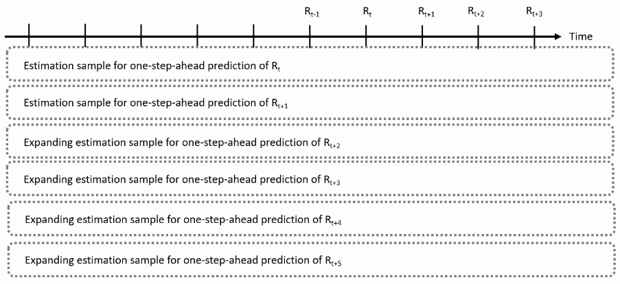
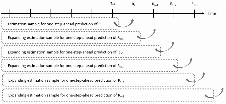
Expanding window estimation

Use all available returns at the time of prediction

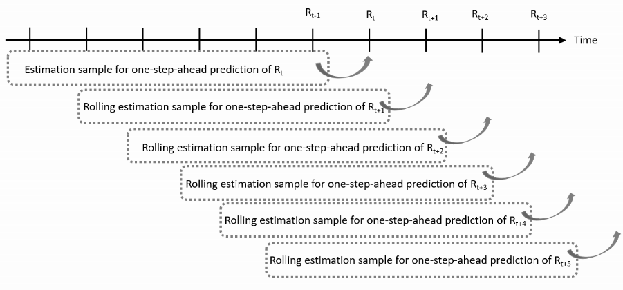
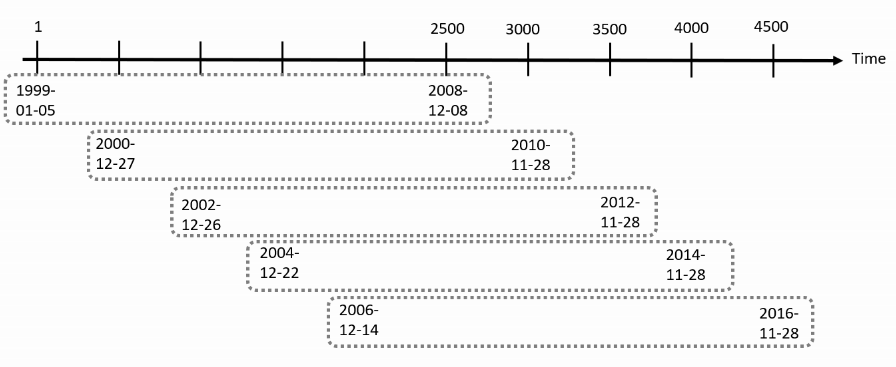
Moving window estimation

Only use a fixed number of the most return observations available at the time of prediction

Properties of rolling window estimation

Rolling window lets you adapt to changes in the model parameters
Computational cost of ugarchroll() is the loop across prediction times:
- Can be reduced by re-estimate the model at a lower frequency than the frequency of prediction

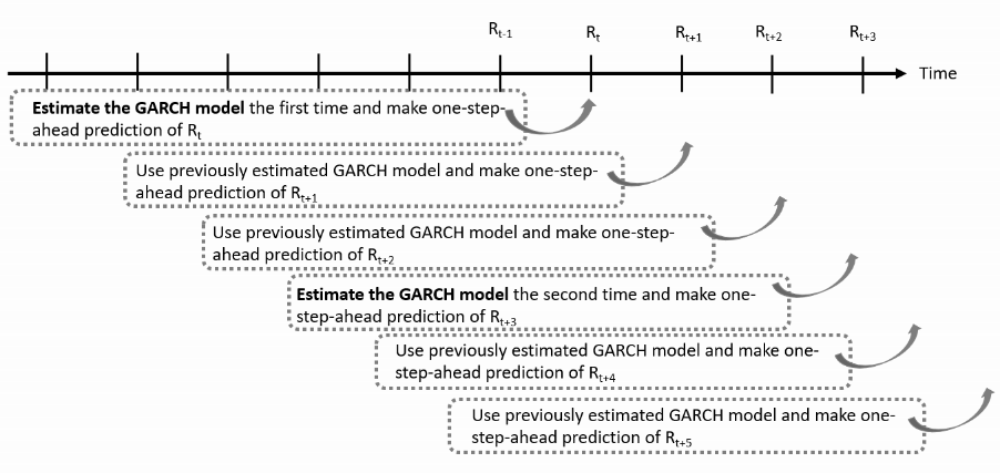
Rolling and re-estimation

Reduce the computational cost by estimating the model every $K$ observations

Function ugarchroll

garchroll <- ugarchroll(tgarchspec, data = EURUSDret, n.start = 2500,
                        refit.window = "moving", refit.every = 500)

Arguments to specify:

GARCH specification used
data : return data to use
n.start: the size of the initial estimation sample
refit.window: how to change that sample through time: "moving" or "expanding
refit.every: how often to re-estimate the model

Example on the Jan 1999-Dec 2018 daily EUR/USD returns

For the 4961 EUR/USD returns with 4961 observations, starting on 1999-01-05 and using a moving estimation window of 2500 observations:

Output of changing parameters

Method coef() produces a list with the estimated coefficients for each estimation

coef(garchroll)[[1]]

$index
"2008-12-08"

$coef
            Estimate   Std. Error     t value  Pr(>|t|)
mu     -1.480000e-04 1.330915e-04 -1.11201737 0.2661307
ar1    -2.953484e-03 1.985344e-02 -0.14876432 0.8817396
omega   7.498928e-08 5.587618e-06  0.01342062 0.9892922
alpha1  2.805079e-02 6.401139e-02  0.43821564 0.6612300
beta1   9.709400e-01 6.080197e-02 15.96889122 0.0000000
shape   1.098068e+01 2.609293e+01  0.42082981 0.6738794

Changes between estimation windows

coef(garchroll)[[1]]$coef # 2008-12-08

            Estimate   Std. Error     t value  Pr(>|t|)
omega   7.498928e-08 5.587618e-06  0.01342062 0.9892922
alpha1  2.805079e-02 6.401139e-02  0.43821564 0.6612300
beta1   9.709400e-01 6.080197e-02 15.96889122 0.0000000

coef(garchroll)[[5]]$coef # 2016-11-28

            Estimate   Std. Error      t value     Pr(>|t|)
omega   8.982527e-08 2.639680e-05  0.003402885 9.972849e-01
alpha1  4.149787e-02 2.550381e-01  0.162712424 8.707449e-01
beta1   9.573885e-01 2.195782e-01  4.360125676 1.299878e-05

What is the rolling predicted mean and volatility?

For the EUR/USD returns with n.start = 2500, the first prediction is for observation 2501, namely 2008-12-09:

Method as.data.frame()

preds <- as.data.frame(garchroll)
head(preds, 3)

                      Mu      Sigma Skew    Shape Shape(GIG)      Realized
2008-12-09 -8.271288e-05 0.01196917    0 10.98068          0  0.0003864884
2008-12-10 -1.495786e-04 0.01179742    0 10.98068          0 -0.0066799754
2008-12-11 -1.287079e-04 0.01167929    0 10.98068          0 -0.0203099142

Note:

preds$Mu: series of predicted mean values
preds$Sigma: series of predicted volatility values

Predicted volatilities

garchvol <- xts(preds$Sigma, order.by = as.Date(rownames(preds)))
plot(garchvol)

Accuracy of rolling predictions

preds <- as.data.frame(garchroll)
head(preds)

                      Mu      Sigma Skew    Shape Shape(GIG)      Realized
2008-12-09 -8.271288e-05 0.01196917    0 10.98068          0  0.0003864884
2008-12-10 -1.495786e-04 0.01179742    0 10.98068          0 -0.0066799754
2008-12-11 -1.287079e-04 0.01167929    0 10.98068          0 -0.0203099142
2008-12-12 -8.845214e-05 0.01199756    0 10.98068          0 -0.0041201588
2008-12-15 -1.362683e-04 0.01184438    0 10.98068          0 -0.0230532787
2008-12-16 -8.034966e-05 0.01228900    0 10.98068          0 -0.0105720492

Evaluate accuracy of preds$Mu and preds$Sigma by comparing with preds$Realized

Mean squared prediction error for the mean

# Prediction error for the mean
e  <- preds$Realized - preds$Mu  
mean(e ^ 2)

3.867998e-05

Mean squared prediction error for the variance

# Prediction error for the mean
e  <- preds$Realized - preds$Mu  

# Prediction error for the variance
d  <- e ^ 2 - preds$Sigma ^ 2 
mean(d ^ 2)

6.974161e-09

Compare two models

Standard GARCH with student t distribution

tgarchspec <- ugarchspec(mean.model = list(armaOrder = c(1, 0)),
     variance.model = list(model = "sGARCH"), distribution.model = "std")
garchroll <- ugarchroll(tgarchspec, data = EURUSDret, n.start = 2500,
                        refit.window = "moving", refit.every = 500)

GJR GARCH with skewed student t distribution

gjrgarchspec <- ugarchspec(mean.model = list(armaOrder = c(1, 0)),
   variance.model = list(model = "gjrGARCH"), distribution.model = "sstd")
gjrgarchroll <- ugarchroll(gjrgarchspec, data = EURUSDret, n.start = 2500,
            refit.window = "moving", refit.every = 500)

Comparison of prediction accuracny

Standard GARCH with student t distribution

preds <- as.data.frame(garchroll)
e  <- preds$Realized - preds$Mu  
d  <- e ^ 2 - preds$Sigma ^ 2 
mean(d ^ 2) # yields 6.974161e-09

GJR GARCH with skewed student t distribution

gjrpreds <- as.data.frame(gjrgarchroll)
e  <- gjrpreds$Realized - gjrpreds$Mu  
d  <- e ^ 2 - gjrpreds$Sigma ^ 2 
mean(d ^ 2) # yields 6.965095e-09

The proof of the pudding is in the eating

GARCH Models in R