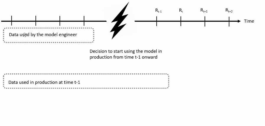
Use the validated GARCH model in production

GARCH Models in R

Kris Boudt

Professor of finance and econometrics

Use in production

Distribution of daily returns per year

New functionality

Use ugarchfilter() for analyzing the recent dynamics in the mean and volatility
Use ugarchforecast() applied to a ugarchspec object (instead of ugarchfit()) object for making the predictions about the future mean and volatility

Example on MSFT returns

msftret: 1999–2017 daily returns.
Suppose the model fitting was done using the returns available at year-end 2010.
You use this model at year-end 2017 to analyze past volatility dynamics and predict future volatility.

Step 1: Defines the final model specification

Fit the best model using the msftret available at year-end 2010:

# Specify AR(1)-GJR GARCH model with skewed student t distribution
garchspec <- ugarchspec(mean.model = list(armaOrder = c(1,0)),
 variance.model = list(model = "gjrGARCH"), distribution.model = "sstd")
# Estimate the model
garchfit <- ugarchfit(data = msftret["/2010-12"], spec = garchspec)

Define progarchspec as the specification to be used in production and use the instruction setfixed(progarchspec) <- as.list(coef(garchfit)):

progarchspec <- garchspec
setfixed(progarchspec) <- as.list(coef(garchfit))

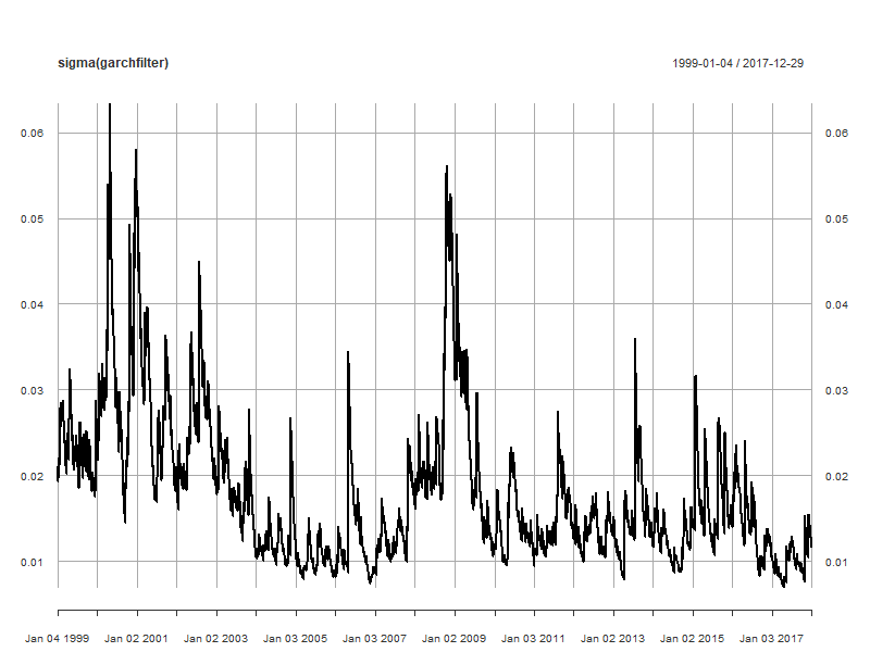
Step 2: Analysis of mean and volatility dynamics

Use the ugarchfilter() function:

garchfilter <- ugarchfilter(data = msftret, spec = progarchspec)
plot(sigma(garchfilter))

Distribution of daily returns per year

Step 3: Make predictions about future returns

garchforecast <- ugarchforecast(data = msftret,
                                fitORspec = progarchspec, 
                                n.ahead = 10) # Make predictions for next ten days

cbind(fitted(garchforecast), sigma(garchforecast))

       2017-12-29 2017-12-29
T+1  0.0004781733 0.01124870
T+2  0.0003610470 0.01132550
T+3  0.0003663683 0.01140171
T+4  0.0003661265 0.01147733
T+5  0.0003661375 0.01155238
T+6  0.0003661370 0.01162688
T+7  0.0003661371 0.01170083
T+8  0.0003661371 0.01177424
T+9  0.0003661371 0.01184712
T+10 0.0003661371 0.01191948

Use in simulation

Instead of applying the complete model to analyze observed returns, you can use it to simulate artificial log-returns:

$$ r_{t} = \log(P_{t}) - \log(P_{t-1}) $$

Useful to assess the randomness in future returns and the impact on prices, since the future price equals:

$$ P_{t + h} = P_{t} \exp(r_{t + 1} + r_{t + 2} + \ldots + r_{t + h}) $$

Step 1: Calibrate the simulation model

Use the log-returns in the estimation

# Compute log returns
msftlogret <- diff(log(MSFTprice))[-1]

Estimate the model and assign model parameters to the simulation model

garchspec <- ugarchspec(mean.model = list(armaOrder = c(1, 0)),
                        variance.model = list(model = "gjrGARCH"),
                        distribution.model = "sstd")
# Estimate the model
garchfit <- ugarchfit(data = msftlogret, spec = garchspec)

# Set that estimated model as the model to be used in the simulation
simgarchspec <- garchspec
setfixed(simgarchspec) <- as.list(coef(garchfit))

Step 2: Run the simulation with `ugarchpath()`

Simulation using the ugarchpath() function requires to choose:

spec : completely specified GARCH model
m.sim : number of time series of simulated returns you want
n.sim: number of observations in the simulated time series (e.g. 252)
rseed : any number to fix the seed used to generate the simulated series (needed for reproducibility)

simgarch <- ugarchpath(spec = simgarchspec, m.sim = 4,
                       n.sim = 10 * 252, rseed = 12345)

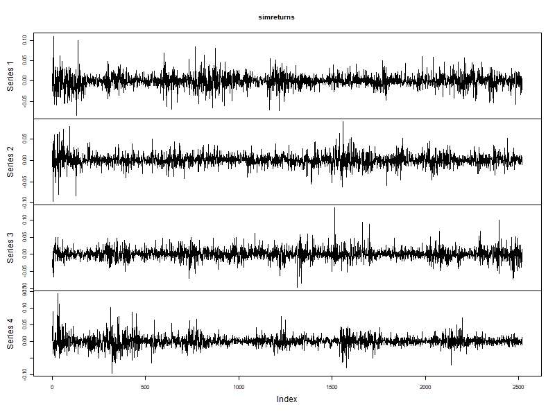
Step 3: Analysis of simulated returns

Method fitted() provides the simulated returns:

simret <- fitted(simgarch)
plot.zoo(simret)

Simulated returns

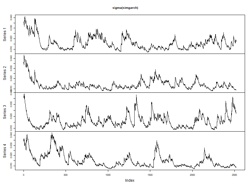
Analysis of simulated volatility

plot.zoo(sigma(simgarch))

Simulated volatility

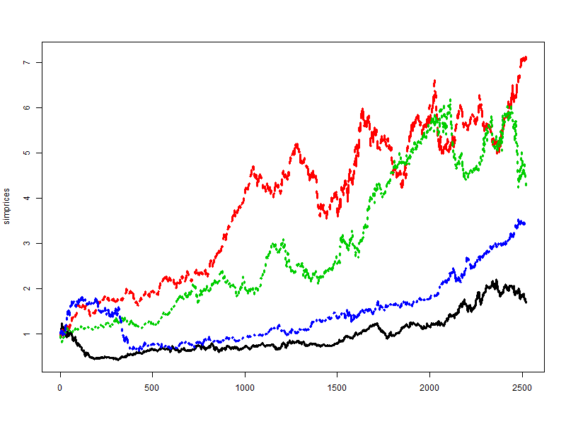
Analysis of simulated prices

Plotting 4 simulations of 10 years of stock prices, with initial price set at 1:

simprices <- exp(apply(simret, 2, "cumsum"))
matplot(simprices, type = "l", lwd = 3)

Simulated prices

Time to practice with setfixed(), ugarchfilter(), ugarchforecast() and ugarchpath()

GARCH Models in R